Prep: Intro to corrections and uncertainties
Overview
Teaching: 20 min
Exercises: 0 minQuestions
How can simulation be used reliably in physics analyses?
How are algorithm efficiencies measured in data and simulation?
How can efficiency differences be corrected?
How do analysts handle uncertainties on corrections?
Objectives
Learn about common issues in matching simulation to data.
Learn some basic methods for computing algorithm efficiencies in CMS.
Learn to apply scale factors to correct simulation.
Essentially all CMS analyses rely on simulation. Whether to simulate a new physics signal or Standard Model processes, it is imperative that simulation reliably reproduces data. Each algorithm that is designed to select events or physics objects must be applied to both data and simulation, so there is always a risk of performance differing between the two. This is quantified by measuring the efficiency for certain objects to be selected by the algorithm. Differences in efficiency between data and simulation are corrected using scale factors.
CMS Analysts regularly evaluate the following algorithms for differences in efficiency between data and simulation:
- Trigger selection
- Object reconstruction (typical for electrons and photons)
- Object identification criteria (typical for all leptons and photons)
- Object isolation criteria (typical for all leptons and photons)
- Jet identification algorithms (b tagging, heavy particle tagging, quark-vs-gluon, etc)
- Custom analysis algorithms
What is efficiency?
Efficiency typically means (number of objects of type X passing algorithm Y) / (number of objects of type X)
Measuring efficiency in data
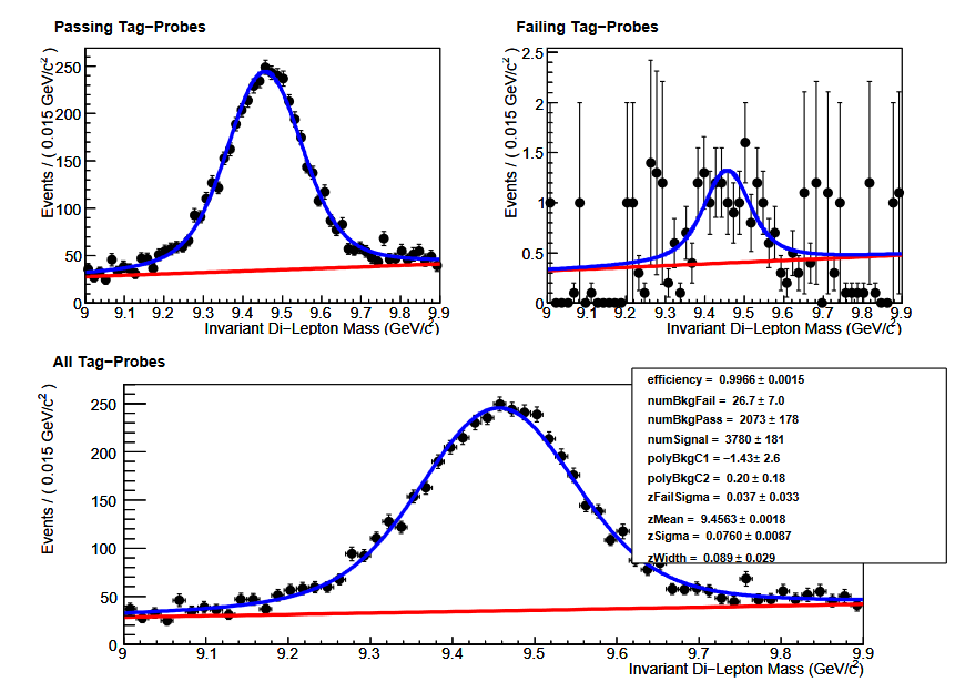
Measuring an algorithm’s efficiency is most complicated in data, because we want to study only “objects of type X”. This might mean “electrons”, “muons”, “b quark jets”, etc, and we have learned how it is difficult to precisely identify these objects in data. But we can bring in physics knowledge to help construct collections of certain particles. The common method of measuring lepton-related efficiencies in data is called tag and probe.
In CMS, tag and probe methods typically use Z boson or J/psi meson resonances that decay into 2 same-flavor leptons. One lepton serves as the “tag” and the other is the “probe”. An event selected for tag and probe has 2 main characteristics:
- tag lepton passes various “tight” quality requirements for trigger filters, identification, and isolation
- dilepton mass from the tag and probe leptons lies within a narrow J/psi or Z mass winder
In events with these characteristics, we can be reasonably sure based on physics that the “probe” lepton is a “real” lepton, and in fact we can do even better by actually fitting the J/psi or Z mass peak to determine the number of events in our calculation. The probe lepton’s properties can then be used to determine the efficiency for essentially any lepton-related algorithm! For example, efficiency for the tight identification working point would be (number of tight probes in the Z peak / total number of probes in the Z peak).
The figure below shows an example of tag and probe using the Upsilon resonance to measure the global muon identification efficiency for muons with momentum between 6 and 20 GeV. Obviously the efficiency is quite high (as expected) since post probes pass the identification criteria. Tag and probe is the standard technique in CMS for measuring electron and muon efficiencies for all algorithms, typically scanning over various momentum and pseudorapidity ranges.
Measuring efficiency in simulation
In simulation, the tag and probe process can certainly be repeated by selecting events using the same criteria as for data. In order to correct the efficiency in simulation to match the efficiency in data it is best if they are computing using the same technique.
For some algorithms, such as b quark jet identification, efficiency for a specific simulated smaple can be measured directly using the truth information stored in the simulation. For b quark tagging, the relevant efficiencies are defined as:
- b efficiency = [number of “real b jets” (jets spatially matched to generator-level b hadrons) tagged as b jets] / [number of real b jets]
- c efficiency = [number of “real c jets” (jets spatially matched to generator-level c hadrons) tagged as c jets] / [number of real c jets]
- light/gluon efficiency (often called “mistag rate”) = [number of “real light/gluon jets” (jets spatially matched to generator-level light hadrons) tagged as light/gluon jets] / [number of real light/gluon jets]
These values are typically computed as functions of the momentum or pseudorapidity of the jet and are computed by analyzers for simulated samples with kinematics relevant to their analysis. In POET, a BTagging module has been provided for calculating efficiencies.
As an example, efficiencies for the CSV Medium working point in the top quark pair sample have been computed and stored in lookup function in PatJetAnalyzer.cc. The CSV algorithm has a b-quark efficiency of ~60% and a light quark mistag rate of ~1%, as advertised.
double PatJetAnalyzer::getBtagEfficiency(double pt){
  if(pt < 25) return 0.263407;
  else if(pt < 50) return 0.548796;
  else if(pt < 75) return 0.656801;
  ...etc...
  else if(pt < 400) return 0.625296;
  else return 0.394916;
}

double PatJetAnalyzer::getLFtagEfficiency(double pt){
  if(pt < 25) return 0.002394;
  else if(pt < 50) return 0.012683;
  else if(pt < 75) return 0.011459;
  ...etc...
  else if(pt < 400) return 0.014760;
  else return 0.011628;
}

Scale factors
Any differences between efficiencies in data and simulation should be corrected using scale factors.
What is a scale factor?
In a given bin of object momentum and pseudorapidity (or other criteria), the scale factor = (efficiency in data) / (efficiency in simulation).
Scale factors inherit the binning of the efficiency measurements, however they are made. For example, the figure below shows the efficiencies in data and simulation for tight muon identification in 2010 data. The corresponding scale factors would be the ratio of the black point to the red point in each bin.

Scale factors are typically applied to simulation using event weights. If a certain scale factor is 1.05, the number of simulated events in that bin should be increased by 5% by giving each individual event a weight of 1.05 instead of 1.
Uncertainties
All scale factors carry uncertainties. Statistical uncertainties arise from the limited number of events available to make the efficiency measurements. Systematic uncertaities can come from a variety of sources, such as:
- Alternate simulated samples
- Alternate efficiency measurement methods
- Alternate fitting functions when fits are used
CMS analysts apply uncertainties in two ways, either as rate uncertainties or shape uncertainties. Rate uncertainties are best for scale factors with very small uncertainties, or uncertainties that are essentially stable for the majority of events in an analysis. For lepton scale factors it is common to assign an uncertainty of 1-2% in all bins. For b tagging and many other scale factors is it more effective to use a shape uncertainty: the scale factor values are shifted up or down according to their uncertainties and 3 versions of the analysis histograms are constructed. An example is shown below for b quark tagging: the uncertainty on the scale factor can be mapped to an uncertainty on the b quark jet momentum using the shape uncertainty concept.
Later in the hands-on exercise and challenge we will practice applying scale factors and working with shape uncertainties.
Key Points
All CMS simulations must be corrected so that algorithm performance matches in data and simulation.
Efficiencies are measured in data using physics knowledge to isolate groups of common objects, such as Z boson tag-and-probe.
Efficiencies in simulation can also be measured using particle truth information.
Scale factors are ratios of efficiency in data to efficiency in simulation, and are applied using event weights.
All scale factor corrections carry either rate or shape uncertainties.
Demo: Muon corrections
Overview
Teaching: 12 min
Exercises: 0 minQuestions
How to correct biased muon momentum?
Objectives
Learn how to apply muon momentum scale corrections to data and MC.
There are misalignments in the CMS detector that make the reconstruction of muon momentum biased. The CMS reconstruction software does not fully correct these misalignments and additional corrections are needed to remove the bias. Correcting the misalignments is important when precision measurements are done using the muon momentum, because the bias in muon momentum will affect the results.
The Muon Momentum Scale Corrections
The Muon Momentum Scale Corrections, also known as the Rochester Corrections, are available in the MuonCorrectionsTool. The correction parameters have been extracted in a two step method. In the first step, initial corrections are obtained in bins of the charge of the muon and the η and ϕ coordinates of the muon track. The reconstruction bias in muon momentum depends on these variables. In the second step, the corrections are fine tuned using the mass of the Z boson.
The corrections for data and Monte Carlo (MC) are different since the MC events start with no biases but they can be induced during the reconstruction. Corrections have been extracted for both data and MC events.
In this example, the Run1 Rochester Corrections are used with a 2012 dataset and a MC dataset. The official code for the Rochester Corrections can be found in the directory RochesterCorrections. The example code for applying the corrections is in the Test directory.
Applying the corrections to data and MC
Let’s start by opening ROOT in a terminal and compiling the official corrections code by running the following lines.
cd MuonCorrectionsTool
root
.L RochesterCorrections/muresolution.cc++
.L RochesterCorrections/rochcor2012wasym.cc++
Then let’s take a look at Analysis.C which is where we apply the corrections.
The main function of Analysis.C is simply used for calling the applyCorrections function which takes as a parameter the name of the ROOT-file (without the .root-part), path to the ROOT-file and a boolean value of whether the file contains data (true) or MC (false). The data file is now commented because it would take too much time to run it during the workshop.
void Analysis::main()
{
  // Data
  // applyCorrections("Run2012BC_DoubleMuParked_Muons", "root://eospublic.cern.ch//eos/opendata/cms/derived-data/AOD2NanoAODOutreachTool/Run2012BC_DoubleMuParked_Muons.root", true);

  // MC
  applyCorrections("ZZTo2e2mu", "root://eospublic.cern.ch//eos/opendata/cms/upload/stefan/HiggsToFourLeptonsNanoAODOutreachAnalysis/ZZTo2e2mu.root", false);
}
The first thing applyCorrections does is create a TTree from the ROOT-file. Then variables for holding the values read from the tree are created and branch addresses are set so that the variables are populated when looping over events. New branches for the corrected values, an output file and a few variables needed for the corrections are also created.
int applyCorrections(string filename, string pathToFile, bool isData) {
  // Create TTree from ROOT file
  TFile *f1 = TFile::Open((pathToFile).c_str());
  TTree *DataTree = (TTree*)f1->Get("Events");
Next, we loop over the events and apply the corrections. We are later going to do an exercise to make sure the corrections have been applied correctly. We are going to need the invariant mass of μ+μ-, which is why the events are filtered to muon pairs with opposite charges and the invariant mass is computed.
// Loop over events
  Int_t nEntries = (Int_t)DataTree->GetEntries();

  for (Int_t k=0; k<nEntries; k++) {
    DataTree->GetEntry(k);

    // Select events with exactly two muons
    if (nMuon == 2 ) {
      // Select events with two muons of opposite charge
      if (Muon_charge[0] != Muon_charge[1]) {

        // Compute invariant mass of the dimuon system
        Dimuon_mass = computeInvariantMass(Muon_pt[0], Muon_pt[1], Muon_eta[0], Muon_eta[1], Muon_phi[0], Muon_phi[1], Muon_mass[0], Muon_mass[1]);
        bDimuon_mass->Fill();
We then loop over the muons in an event and create a TLorentzVector for each muon. The functions for applying the Rochester Corrections take as a parameter a TLorentzVector which is a four-vector that describes the muons momentum and energy. As mentioned earlier, the muon momentum scale corrections are different for data and MC and therefore there are separate functions for both: momcor_data and momcor_mc. These functions can be found in rochcor2012wasym.cc if you want to take a closer look at them.
        // Loop over muons in event
        for (UInt_t i=0; i<nMuon; i++) {

          // Fill positive and negative muons eta branches
          if (Muon_charge[i] > 0) {
            Muon_eta_pos[i] = Muon_eta[i];
            bMuon_eta_pos->Fill();
          } else {
            Muon_eta_neg[i] = Muon_eta[i];
            bMuon_eta_neg->Fill();
          }

          // Create TLorentzVector
          TLorentzVector mu;
          mu.SetPtEtaPhiM(Muon_pt[i], Muon_eta[i], Muon_phi[i], Muon_mass[i]);

          // Apply the corrections
          if (isData) {
            rmcor.momcor_data(mu, Muon_charge[i], runopt, qter);
          } else {
            rmcor.momcor_mc(mu, Muon_charge[i], ntrk, qter);
          }
The corrected values are then saved to the new branches and the corrected invariant mass is computed. The new tree is filled and written to the output file.
          // Save corrected values
          Muon_pt_cor[i] = mu.Pt();
          bMuon_pt_cor->Fill();
          Muon_eta_cor[i] = mu.Eta();
          bMuon_eta_cor->Fill();
          Muon_phi_cor[i] = mu.Phi();
          bMuon_phi_cor->Fill();
          Muon_mass_cor[i] = mu.M();
          bMuon_mass_cor->Fill();
        }

        // Compute invariant mass of the corrected dimuon system
        Dimuon_mass_cor = computeInvariantMass(Muon_pt_cor[0], Muon_pt_cor[1], Muon_eta_cor[0], Muon_eta_cor[1], Muon_phi_cor[0], Muon_phi_cor[1], Muon_mass_cor[0], Muon_mass_cor[1]);
        bDimuon_mass_cor->Fill();

      }
    }
    //Fill the corrected values to the new tree
    DataTreeCor->Fill();
  }

  //Save the new tree
  DataTreeCor->Write();
Compile and run Analysis.C by running the following lines in your ROOT-terminal. You will get a bunch of warnings but you can safely ignore them.
.L RochesterCorrections/Test/Analysis.C+
Analysis pf
pf.main()
And that’s it! As a result you can find ZZTo2e2mu_Cor.root in the Test directory. The file contains both corrected and uncorrected values.
Key Points
Rochester corrections are used to scale the muon momentum so that simulation better matches data.
Demo: Heavy flavor tagging
Overview
Teaching: 12 min min
Exercises: minQuestions
How are b hadrons identified in CMS
Objectives
Understand the basics of heavy flavor tagging
Learn to access tagging information in AOD files
Jet reconstruction and identification is an important part of the analyses at the LHC. A jet may contain the hadronization products of any quark or gluon, or possibly the decay products of more massive particles such as W or Higgs bosons. Several “b tagging” algorithms exist to identify jets from the hadronization of b quarks, which have unique properties that distinguish them from light quark or gluon jets.
B Tagging Algorithms
Tagging algorithms first connect the jets with good quality tracks that are either associated with one of the jet’s particle flow candidates or within a nearby cone. Both tracks and “secondary vertices” (track vertices from the decays of b hadrons) can be used in track-based, vertex-based, or “combined” tagging algorithms. The specific details depend upon the algorithm use. However, they all exploit properties of b hadrons such as:
- long lifetime,
- large mass,
- high track multiplicity,
- large semileptonic branching fraction,
- hard fragmentation fuction.
Tagging algorithms are Algorithms that are used for b-tagging:
- Track Counting: identifies a b jet if it contains at least N tracks with significantly non-zero impact parameters.
- Jet Probability: combines information from all selected tracks in the jet and uses probability density functions to assign a probability to each track
- Soft Muon and Soft Electron: identifies b jets by searching for a lepton from a semi-leptonic b decay.
- Simple Secondary Vertex: reconstructs the b decay vertex and calculates a discriminator using related kinematic variables.
- Combined Secondary Vertex: exploits all known kinematic variables of the jets, information about track impact parameter significance and the secondary vertices to distinguish b jets. This tagger became the default CMS algorithm.
These algorithms produce a single, real number (often the output of an MVA) called a b tagging “discriminator” for each jet. The more positive the discriminator value, the more likely it is that this jet contained b hadrons.
Accessing tagging information
In PatJetAnalyzer.cc we access the information from the Combined Secondary Vertex (CSV) b tagging algorithm and associate discriminator values with the jets.
The CSV values are stored in a separate collection in the AOD files called a JetTagCollection, which is effectively a vector of associations between jet references and
float values (such as a b-tagging discriminator). During the creation of pat::Jet objects, this information is merged into the jets so that the discriminators can be accessed with a dedicated member function (similar merging is done for other useful associations like generated jets and jet flavor in simulation!).
For examples of working with b tags and RECO jets, see last year’s lesson.
#include "DataFormats/PatCandidates/interface/Jet.h"

Handle<std::vector<pat::Jet>> myjets;
iEvent.getByLabel(jetInput, myjets); // jetInput opens "selectedPatJetsAK5PFCorr"

for (std::vector<pat::Jet>::const_iterator itjet=myjets->begin(); itjet!=myjets->end(); ++itjet){

  jet_btag.push_back(itjet->bDiscriminator("combinedSecondaryVertexBJetTags"));

}
We can investigate at the b tag information in a dataset using ROOT.
$ root -l myoutput.root // you produced this earlier in hands-on exercise #2
[0] _file0->cd("myjets");
[1] Events->Draw("jet_btag");
The discriminator values for jets with kinematics in the correct range for this algorithm lie between 0 and 1. Other jets that do not have a valid discriminator value pick up values of -1, -9, or -999.
Working points
A jet is considered “b tagged” if the discriminator value exceeds some threshold. Different thresholds will have different efficiencies for identifying true b quark jets and for mis-tagging light quark jets. As we saw for muons and other objects, a “loose” working point will allow the highest mis-tagging rate, while a “tight” working point will sacrifice some correct-tag efficiency to reduce mis-tagging. The CSV algorithm has working points defined based on mis-tagging rate:
- Loose = ~10% mis-tagging = discriminator > 0.244
- Medium = ~1% mis-tagging = discriminator > 0.679
- Tight = ~0.1% mis-tagging = discriminator > 0.898
The method used to calculate these efficiencies was described in the introductory episode. The figures below show examples of the b and light quark efficiencies and scale factors as a function of jet momentum for the CSV Medium working point (read more).


Applying scale factors
Scale factors to increase or decrease the number of b-tagged jets in simulation can be applied in a number of ways, but typically involve weighting simulation events based on the efficiencies and scale factors relevant to each jet in the event. Scale factors for the CSV algorithm are available for Open Data and involve extracting functions from a comma-separated-values file. Details and usage reference can be found at these references:
In POET, the scale factor functions in the comma-separated-values file for the Medium working point have been implemented in PatJetAnalyzer.cc. The scale factor is a single numerical value calculated from a function of the corrected jet momentum:
double PatJetAnalyzer::getBorCtagSF(double pt, double eta){
  if (pt > 670.) pt = 670;
  if(fabs(eta) > 2.4 or pt<20.) return 1.0;

  return 0.92955*((1.+(0.0589629*pt))/(1.+(0.0568063*pt)));
}
The most commonly used method to apply scale factors is Method 1a, and it has been implemented in POET. This is an event weight method of applying a correction, so the final result is an event weight to be stored for later in the analysis, along with extra event weights to describe the uncertainty.
The method relies on 4 pieces of information for each jet in simulation:
- Tagging status: does this jet pass the discriminator threshold for a given working point?
- Flavor (b, c, light): accessed using a
pat::Jetmember function calledpartonFlavour(). - Efficiency: accessed from the lookup functions based on the jet’s momentum.
- Scale factor: accessed from the helper functions based on the jet’s momentum.
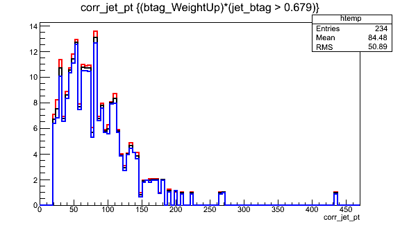
Each jet then contributes to the event weight based on these four features. For example, jets that pass the discriminator threshold and are b quark jets contribute the following factor to variables called MC, which appears as P(MC) in the reference TWiki, and btagWeight, which appears as P(DATA) in the reference TWiki.
hadronFlavour = itjet->partonFlavour();
corrpt = corr_jet_pt.at(value_jet_n);

if (jet_btag.at(value_jet_n) > 0.679){
  if(abs(hadronFlavour) == 5){
    eff = getBtagEfficiency(corrpt);
    SF = getBorCtagSF(corrpt, jet_eta.at(value_jet_n));
    SFu = SF + uncertaintyForBTagSF(corrpt, jet_eta.at(value_jet_n));
    SFd = SF - uncertaintyForBTagSF(corrpt, jet_eta.at(value_jet_n));
  }
  // ... repeat for c and light quark jets...
  MC *= eff;
  btagWeight *= SF * eff;
  btagWeightUp *= SFu * eff;
  btagWeightDn *= SFd * eff;
}
//...similar for non-tagged jets...
After the jet loop, the reference TWiki defines the weight as P(DATA)/P(MC):
btagWeight = (btagWeight/MC);
btagWeightUp = (btagWeightUp/MC);
btagWeightDn = (btagWeightDn/MC);
The weight and its uncertainties are all stored in the tree for use later in filling histograms.
Key Points
Tagging algorithms separate heavy flavor jets from jets produced by the hadronization of light quarks and gluons
Tagging algorithms produce a disriminator value for each jet that represents the likelihood that the jet came from a b hadron
Each tagging algorithm has recommended ‘working points’ (discriminator values) based on a misidentification probability for light-flavor jets
Demo: Jet corrections
Overview
Teaching: 12 min
Exercises: 0 minQuestions
How are data/simulation differences dealt with for jet energy?
Objectives
Learn about typical differences in jet energy scale and resolution between data and simulation
Learn how JEC and JER corrections can be applied to OpenData jets
Access uncertainties in both JEC and JER
Unsurprisingly, the CMS detector does not measure jet energies perfectly, nor do simulation and data agree perfectly! The measured energy of jet must be corrected so that it can be related to the true energy of its parent particle. These corrections account for several effects and are factorized so that each effect can be studied independently. All of the corrections in this section are described in “Jet Energy Scale and Resolution” papers by CMS:
Correction levels
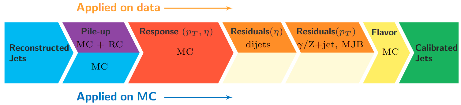
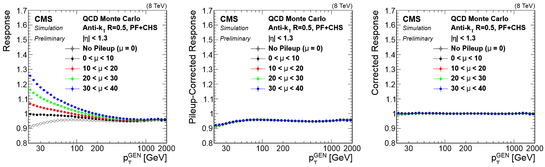
Particles from additional interactions in nearby bunch crossings of the LHC contribute energy in the calorimeters that must somehow be distinguished from the energy deposits of the main interaction. Extra energy in a jet’s cone can make its measured momentum larger than the momentum of the parent particle. The first layer (“L1”) of jet energy corrections accounts for pileup by subtracting the average transverse momentum contribution of the pileup interactions to the jet’s cone area. This average pileup contribution varies by pseudorapidity and, of course, by the number of interactions in the event.
The second and third layers of corrections (“L2L3”) correct the measured momentum to the true momentum as functions of momentum and pseudorapidity, bringing the reconstructed jet in line with the generated jet. These corrections are derived using momentum balancing and missing energy techniques in dijet and Z boson events. One well-measured object (ex: a jet near the center of the detector, a Z boson reconstructed from leptons) is balanced against a jet for which corrections are derived.
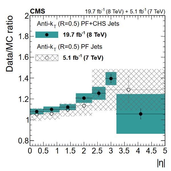
All of these corrections are applied to both data and simulation. Data events are then given “residual” corrections to bring data into line with the corrected simulation. A final set of flavor-based corrections are used in certain analyses that are especially sensitive to flavor effects. The figure below shows the result of the L1+L2+L3 corrections on the jet response.
Jet Energy Resolution
Jet Energy Resolution (JER) corrections are applied after JEC on strictly MC simulations. Unlike JEC, which adjusts the mean of the momentun response distribution, JER adjusts the width of the distribution. The ratio of reconstructed transverse momentum to true (generated) transverse momentum forms a Gaussian distributions – the width of this Gaussian is the JER. In data, where no “true” pT is available, the JER is measured using photon/Z + jet events where the jet recoils against the photon or Z boson, both of which can be measured quite precisely in the CMS detector. The JER is typically smaller in simulation than in data, leading to scale factors that are larger than 1. These scale factors, along with their uncertainties, are accessible in POET in the jet analyzers. They are applied using two methods:
- Adjusting the ratio of reconstructed to generated momentum using the scale factor (if a well-matched generated jet is found),
- Randomly smearing the momentum using a Gaussian distribution based on the resolution and scale factor (if no generated jet is found).
Applying JEC and JER
The jet energy corrections and Type-1 MET corrections can be applied to RECO jets while making PAT jets. To do this we will use the ‘addJetCollection’
process in python/poet_cfg.py. You can see that simulation and data use slightly different lists of correction levels as we discussed.
# Choose which jet correction levels to apply
jetcorrlabels = ['L1FastJet','L2Relative','L3Absolute']
if isData:
  # For data we need to remove generator-level matching processes
  runOnData(process, ['Jets','METs'], "", None, [])
  jetcorrlabels.append('L2L3Residual')

# Configure the addJetCollection tool
# This process will make corrected jets with b-tagging included, and will make Type1-corrected MET
process.ak5PFJets.doAreaFastjet = True
addJetCollection(process,cms.InputTag('ak5PFJets'),
    'AK5', 'PFCorr',
    doJTA        = True,
    doBTagging   = True,
    jetCorrLabel = ('AK5PF', cms.vstring(jetcorrlabels)),
    doType1MET   = True,
    doL1Cleaning = False,
    doL1Counters = False,
    doJetID      = True,
    jetIdLabel   = "ak5",
    )
In PatJetAnalyzer.cc the corrected momenta and energy come for free! For extra information we can access the uncorrected jet
and store some of its features as well.
for (std::vector<pat::Jet>::const_iterator itjet=myjets->begin(); itjet!=myjets->end(); ++itjet){
  pat::Jet uncorrJet = itjet->correctedJet(0);

  // itjet is the corrected jet and uncorrJet is the raw jet
}
The JER corrections must be accessed from a text file and applied on top of the corrected jets. The text file is
read in using the SimpleJetCorrector class which provides a correction() member function that will evaluate the formula
provided in the text file given the necessary variables (in this case: momentum, pseudorapidity, and number of pileup vertices).
In the constructor function PatJetAnalyzer::PatJetAnalyzer:
jerResName_ = iConfig.getParameter<edm::FileInPath>("jerResName").fullPath(); // JER Resolutions

JetCorrectorParameters *ak5PFPar = new JetCorrectorParameters(jerResName_);
jer_ = boost::shared_ptr<SimpleJetCorrector>( new SimpleJetCorrector(*ak5PFPar) );
We can now use jer_->correction() to access the jet’s momentum resolution in simulation. In the code snippet below you can see “scaling” and “smearing” versions of applying the JER scale factors, depending
on whether or not this pat::Jet had a matched generated jet. The random smearing application uses a reproducible seed for the random number generator based on the inherently random azimuthal angle of the jet.
Note: this code snippet is simplified by removing lines for handling uncertainties – that’s coming below!
for (std::vector<pat::Jet>::const_iterator itjet=myjets->begin(); itjet!=myjets->end(); ++itjet){
  pat::Jet uncorrJet = itjet->correctedJet(0);

  ptscale = 1;
  res = 1;
  if(!isData) {
    std::vector<float> factors = factorLookup(fabs(itjet->eta())); // returns in order {factor, factor_down, factor_up}
    std::vector<float> feta;
    std::vector<float> PTNPU;
    feta.push_back( fabs(itjet->eta()) );
    PTNPU.push_back( itjet->pt() );
    PTNPU.push_back( vertices->size() );

    res = jer_->correction(feta, PTNPU);

    float reco_pt = itjet->pt();
    const reco::GenJet *genJet = itjet->genJet();
    bool smeared = false;

    // Attempt the truth-vs-reco smearing
    if(genJet){
      double deltaPt = fabs(genJet->pt() - reco_pt);
      double deltaR = reco::deltaR(genJet->p4(),itjet->p4());
      if ((deltaR < 0.25) && deltaPt <= 2*reco_pt*res){
        double ptratio = reco_pt/genJet->pt();
        ptscale = max(0.0, ptratio + factors[0]*(1 - ptratio));
        smeared = true;
      }
    }
    // If that didn't work, use Gaussian smearing with a reproducible seed
    if (!smeared && factors[0] > 1) {
      TRandom3 JERrand;

      JERrand.SetSeed(abs(static_cast<int>(itjet->phi()*1e4)));
      ptscale = max(0.0, 1.0 + JERrand.Gaus(0,res)*sqrt(factors[0]*factors[0] - 1.0));
    }
  }
}
The final, definitive jet momentum is the raw momentum multiplied by both JEC and JER corrections! After computing ptscale, we store a variety of corrected and uncorrected kinematic variables for jets passing the momentum threshold:
if( ptscale*itjet->pt() <= min_pt) continue;

jet_pt.push_back(uncorrJet.pt());
// ...other variables...
corr_jet_pt.push_back(ptscale*itjet->pt());
Uncertainties
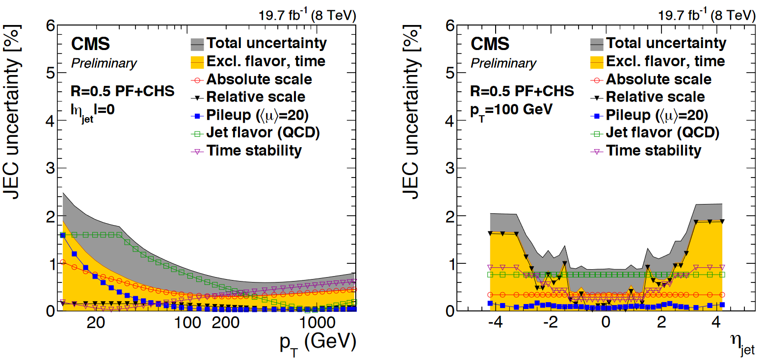
You will have noticed that nested among the JEC and JER code snippets given above were commands related to the uncertainty in these corrections. The JEC uncertainties have several sources, shown in the figure below. The L1 (pileup) uncertainty dominates at low momentum, while the L3 (absolute scale) uncertainty takes over for higher momentum jets. All corrections are quite precise for jets located near the center of the CMS barrel region, and the precision drops as pseudorapidity increases and different subdetectors lose coverage.
The JER uncertainty is evaluated by shifting the scale factors up and down according to the error bars shown in the scale factor figure above. These uncertainties arise from treatment of initial and final state radiation in the data measurement, differences in Monte Carlo tunes across generator platforms, and small non-Gaussian tail effects.
The JEC uncertainty text file is loaded as a JetCorrectionUncertainty object in the PatJetAnalyzer constructor:
jecUncName_ = iConfig.getParameter<edm::FileInPath>("jecUncName").fullPath(); // JEC uncertainties

jecUnc_ = boost::shared_ptr<JetCorrectionUncertainty>( new JetCorrectionUncertainty(jecUncName_) );
This object provides a getUncertainty() function that takes in the jet’s momentum and pseudorapidity and returns an adjustment to the JEC correction factor:
for (std::vector<pat::Jet>::const_iterator itjet=myjets->begin(); itjet!=myjets->end(); ++itjet){
  pat::Jet uncorrJet = itjet->correctedJet(0);

  double corrUp = 1.0;
  double corrDown = 1.0;
  jecUnc_->setJetEta( itjet->eta() );
  jecUnc_->setJetPt( itjet->pt() );
  corrUp = (1 + fabs(jecUnc_->getUncertainty(1)));
  jecUnc_->setJetEta( itjet->eta() );
  jecUnc_->setJetPt( itjet->pt() );
  corrDown = (1 - fabs(jecUnc_->getUncertainty(-1)));
The JER uncertainty is evaluated by calculating a ptscale_up and ptscale_down correction, exactly as shown above for the ptscale correction, but using the shifted scale factors. The uncertainties in JEC and JER are kept separate from each other: when varying JEC, the JER correction is held constant, and vice versa. This results in 5 momentum branches: a central value and two sets of uncertainties:
corr_jet_pt.push_back(ptscale*itjet->pt());
corr_jet_ptUp.push_back(ptscale*corrUp*itjet->pt());
corr_jet_ptDown.push_back(ptscale*corrDown*itjet->pt());
corr_jet_ptSmearUp.push_back(ptscale_up*itjet->pt());
corr_jet_ptSmearDown.push_back(ptscale_down*itjet->pt());
Key Points
Jet energy corrections are factorized and account for many mismeasurement effects
L1+L2+L3 should be applied to jets used for analyses, with residual corrections for data
Jet energy resolution in simulation is typically too narrow and is smeared using scale factors
Jet energy and resolution corrections are sources of systematic error and uncertainties should be evaluated
15 minute break
Overview
Teaching: 0 min
Exercises: 15 minQuestions
Which type of coffee will you drink on your break?
Objectives
Acquire coffee. Drink coffee.
Take a break!
Key Points
Any type of coffee is refreshing after so much concentrated learning.
Advanced objects hands-on
Overview
Teaching: 0 min
Exercises: 40 minQuestions
How can I visualize the effect of the muon corrections?
How do I access other b tagging discriminators?
How do I apply the b tagging scale factors and visualize the uncertainty?
Objectives
Practice plotting histograms in ROOT to view POET histograms.
Implement multiple b taggers and count the number of b-tagged jets
Apply the central and shifted b tagging scale factors
Choose your exercise! Complete exercise #1 on the muon corrections, and then choose one of the options for exercise #2 on b-tagging.
Exercise 1: results of the muon correction
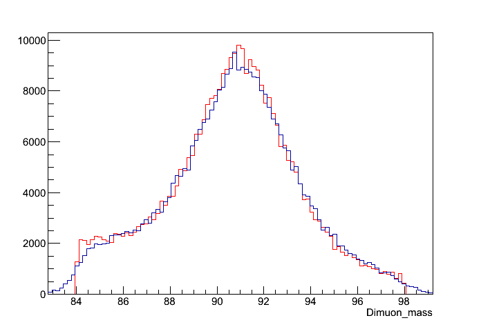
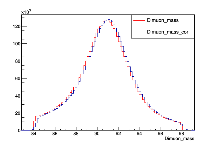
Check that the corrections have been applied correctly by plotting the corrected and uncorrected invariant mass of μ+μ- on the ROOT command line. If everything went right with the corrections, there should be a difference in the invariant masses. Cut the x-axis to be from 84 to 98.
Hint: You can find the branch names of the invariant masses from Analysis.C.
Solution
$ root RochesterCorrections/Test/ZZTo2e2mu_Cor.root
[0] Events->Draw("Dimuon_mass", "Dimuon_mass > 84 && Dimuon_mass < 98")
[1] Events->Draw("Dimuon_mass_cor", "Dimuon_mass > 84 && Dimuon_mass < 98", "hist same"); htemp->SetLineColor(2);
You should get something like this:
An example of what the plot looks like for data:
Exercise 2 option A: alternate b taggers
The statements printed from
addJetCollectionwhen runningpoet_cfg.pyshows the options for strings that can be used in thebdiscriminator()function:The bdiscriminators below will be written to the jet collection in the PATtuple (default is all, see PatAlgos/PhysicsTools/python/tools/jetTools.py) jetBProbabilityBJetTags jetProbabilityBJetTags trackCountingHighPurBJetTags trackCountingHighEffBJetTags simpleSecondaryVertexHighEffBJetTags simpleSecondaryVertexHighPurBJetTags combinedSecondaryVertexBJetTagsAdd 1-2 new branches for alternate taggers and compare those discriminants to CSV.
After editing
PatJetAnalyzer.cc,$ scram b $ cmsRun python/poet_cfg.py False True $ root -l myoutput.root [0] TBrowser bSolution
Let’s add the high purity track counting tagger, which was the most common tagger in 2011. After adding a new array declaration and branch in the top sections of
PatJetAnalyzer.cc, we can callbDiscriminator()for these alternate tagger:// Declarations std::vector<double> jet_btag; std::vector<double> jet_btagTC; // Branches mtree->Branch("jet_btag",&jet_btag); mtree->Branch("jet_btagTC",&jet_btagTC); // inside the jet loop jet_btag.push_back(itjet->bDiscriminator("combinedSecondaryVertexBJetTags")); jet_btag.push_back(itjet->bDiscriminator("trackCountingHighPurBJetTags"));The distributions in ttbar events (excluding events with null values) look remarkably different! The CSV algorithm is a typical “multivariate” discriminant that ranges from 0 to 1 while the track counting discriminant represents a physics-based impact parameter quantity that has a much wider range of values. More information about the various taggers can be found here.
Exercise 2 option B: count medium CSV b tags
Calculate the number of jets per event that are b tagged according to the medium working point of the CSV algorithm. Store a branch called
jet_nCSVMand draw it 3 times, applying the scale factor weights and demonstrating the uncertainty.After editing
PatJetAnalyzer.cc,$ scram b $ cmsRun python/poet_cfg.py False True $ root -l myoutput.root [0] _file0->cd("myjets") [1] Events->Draw("jet_nCSVM","(btagWeight)") [2] Events->Draw("jet_nCSVM","(btagWeightUp)","p hist same") [3] Events->Draw("jet_nCSVM","(btagWeightDown)","p hist same")Solution
We count the number of “Medium CSV” b-tagged jets by summing up the number of jets with discriminant values greater than 0.679. After adding a variable declaration and branch we can sum up the counter:
int jet_nCSVM = 0;
for (std::vector<pat::Jet>::const_iterator itjet=myjets->begin(); itjet!=myjets->end(); ++itjet){

 // ... JEC uncert, JER, storing variables...

 jet_btag.push_back(itjet->bDiscriminator("combinedSecondaryVertexBJetTags"));
 if (itjet->bDiscriminator("combinedSecondaryVertexBJetTags") > 0.679) jet_nCSVM++;
}
Applying the scale factor weight shifts the mean of the distribution down slightly. The uncertainty wraps around the central distribution with a magnitude of approximately 6% in this sample.
Key Points
Muon corrections are a precision adjustment to a dimuon mass histogram.
B tagging scale factors and uncertainties should be considered for any distribution that relies on b-tagged jets
Offline: Advanced object challenge
Overview
Teaching: 0 min
Exercises: 30 minQuestions
How do uncorrected and corrected jet momenta compare?
How large is the JEC uncertainty in different regions?
How large is the JER uncertainty in different regions?
Objectives
Explore the JEC and JER uncertainties using histograms
Practice basic plotting with ROOT
Let’s dig into the JEC and JER corrections and uncertainties by studying their effect on jet momentum histograms.
Run POET
Take some time to run POET using the entire top quark pair test file. In
python/poet_cfg.pyset the number of events to process to -1:#---- Select the maximum number of events to process (if -1, run over all events) process.maxEvents = cms.untracked.PSet( input = cms.untracked.int32(-1) )And run POET using
cmsRun python/poet_cfg.py False True. Great time to read ahead on tomorrow’s lessons!
Open myoutput.root and investigate the range of momentum variation given by the JEC uncertainties by plotting:
- Corrected versus uncorrected jet momentum
- Corrected jet momentum with JEC up and down uncertainties
- Corrected jet momentum with JER up and down uncertainties
Questions:
Is the difference between the raw and corrected momentum larger or smaller than the uncertainty? Which uncertainty dominates?
Repeat these plots with the additional requirement that the jets be “forward” (
abs(jet_eta) > 3.0) How do the magnitudes of the uncertainties compare in this region?
Recall: to draw plots on the ROOT command line use the following syntax:
$ root -l myoutput.root
[0] _file0->cd("myjets");
[1] Events->Draw("jet_pt"); // draw the branch jet_pt
[2] Events->Draw("jet_pt","abs(jet_eta) > 3.0","same"); // draw jet_pt with a cut on jet_eta, on top of the previous plot
[3] Events->Draw("jet_pt","abs(jet_eta) < 3.0","pe same"); // draw jet_pt again with a different cut using points & error bars
To use different line colors and styles in a plot, “right-click” on a histograms and use the “Set Line Attributes” GUI to change the color and style of the lines and markers. Clicking on a different histogram will automatically change which plot’s style the GUI is controlling.
Solutions
Come back tomorrow to go over these plots!
Key Points
Come back for the solutions session tomorrow!
Come back tomorrow morning!
Overview
Teaching: min
Exercises: minQuestions
Objectives
The solutions session for this lesson is schedule for Wednesday at 14:30 CERN time. See you then!
Key Points
Solutions and questions
Overview
Teaching: 40 min
Exercises: 0 minQuestions
How do uncorrected and corrected jet momenta compare?
How large is the JEC uncertainty in different regions?
How large is the JER uncertainty in different regions?
Objectives
Explore the JEC and JER uncertainties using histograms
Practice basic plotting with ROOT
Open myoutput.root and investigate the range of momentum variation given by the JEC uncertainties by plotting:
- Corrected versus uncorrected jet momentum
- Corrected jet momentum with JEC up and down uncertainties
- Corrected jet momentum with JER up and down uncertainties
Questions:
Is the difference between the raw and corrected momentum larger or smaller than the uncertainty? Which uncertainty dominates?
Solution
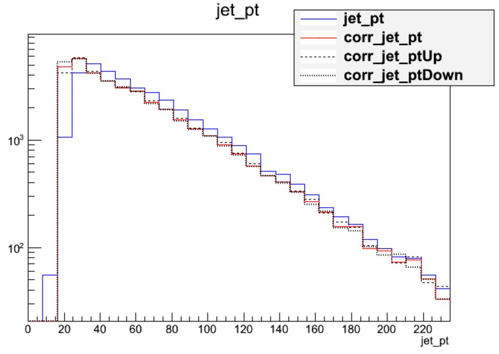
The following plotting commands can be used to draw the four histograms needed to answer the first question:
$ root -l myoutput.root
[1] _file0->cd("myjets");
[2] Events->Draw("jet_pt");
[3] Events->Draw("corr_jet_pt","","hist same");
[4] Events->Draw("corr_jet_ptUp","","hist same");
[5] Events->Draw("corr_jet_ptDown","","hist same");
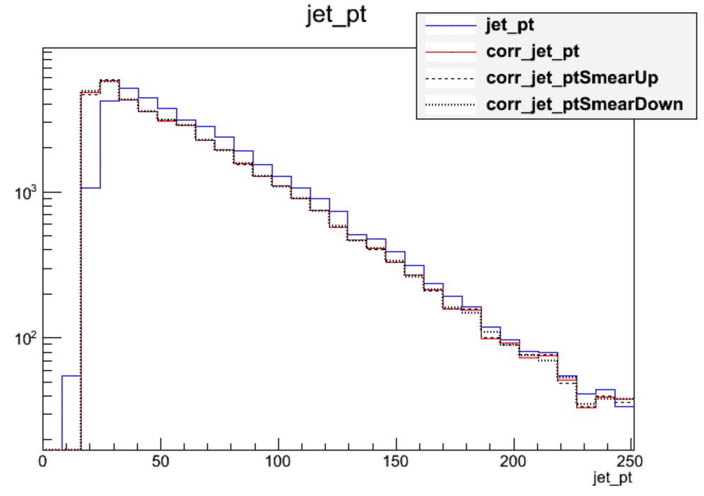
We can see that the corrections are significant, far larger than the uncertainty itself. The first level of correction, for pileup removal, tends to reduce the momentum of the jet. The JER uncertainty can be drawn using similar commands:
This uncertainty is much smaller for the majority of jets! The JER correction is similar to the muon Rochester corrections in that it is most important for analyses requiring higher precision in jet agreement between data and simulation.
Repeat these plots with the additional requirement that the jets be “forward” (
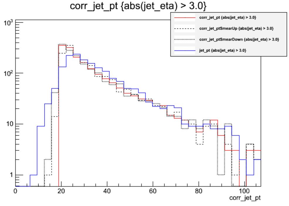
abs(jet_eta) > 3.0) How do the magnitudes of the uncertainties compare in this region?Solution
This time we need to apply cuts to the jets as we draw:
$ root -l myoutput.root
[1] _file0->cd("myjets");
[2] Events->Draw("jet_pt","abs(jet_eta) > 3.0");
[3] Events->Draw("corr_jet_pt","abs(jet_eta) > 3.0","hist same");
[4] Events->Draw("corr_jet_ptUp","abs(jet_eta) > 3.0","hist same");
[5] Events->Draw("corr_jet_ptDown","abs(jet_eta) > 3.0","hist same");
In the endcap region the uncertainty on the JER scale factor has become nearly 20%! So this uncertainty gains almost equal footing with JEC. Many CMS analyses restrict themselves to studying jets in the “central” region of the detector, defined loosely by the tracker acceptance region of
abs(eta) < 2.4precisely to avoid these larger JEC and JER uncertainties.
Key Points
In general, the jet corrections are significant and lower the momenta of the jets with standard LHC pileup conditions.
For most jets, the JEC uncertainty dominates over the JER uncertainty.
In the endcap region of the detector, the JER uncertainty in larger and matches the JEC uncertainty.