Advanced objects hands-on

Overview

Teaching: 0 min
Exercises: 40 min

Questions

• How can I visualize the effect of the muon corrections?

• How do I access other b tagging discriminators?

• How do I apply the b tagging scale factors and visualize the uncertainty?

Objectives

• Practice plotting histograms in ROOT to view POET histograms.

• Implement multiple b taggers and count the number of b-tagged jets

• Apply the central and shifted b tagging scale factors

Choose your exercise! Complete exercise #1 on the muon corrections, and then choose one of the options for exercise #2 on b-tagging.

Exercise 1: results of the muon correction

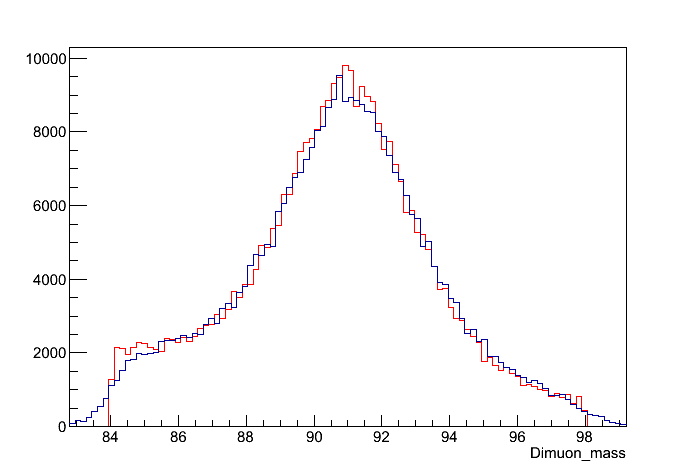
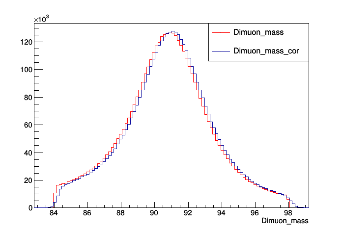
Check that the corrections have been applied correctly by plotting the corrected and uncorrected invariant mass of μ⁺μ^- on the ROOT command line. If everything went right with the corrections, there should be a difference in the invariant masses. Cut the x-axis to be from 84 to 98.

Hint: You can find the branch names of the invariant masses from Analysis.C.

Solution

$ root RochesterCorrections/Test/ZZTo2e2mu_Cor.root
[0] Events->Draw("Dimuon_mass", "Dimuon_mass > 84 && Dimuon_mass < 98")
[1] Events->Draw("Dimuon_mass_cor", "Dimuon_mass > 84 && Dimuon_mass < 98", "hist same"); htemp->SetLineColor(2);

You should get something like this:

An example of what the plot looks like for data:

Exercise 2 option A: alternate b taggers

The statements printed from addJetCollection when running poet_cfg.py shows the options for strings that can be used in the bdiscriminator() function:

The bdiscriminators below will be written to the jet collection in the PATtuple (default is all, see PatAlgos/PhysicsTools/python/tools/jetTools.py)
jetBProbabilityBJetTags
jetProbabilityBJetTags
trackCountingHighPurBJetTags
trackCountingHighEffBJetTags
simpleSecondaryVertexHighEffBJetTags
simpleSecondaryVertexHighPurBJetTags
combinedSecondaryVertexBJetTags

Add 1-2 new branches for alternate taggers and compare those discriminants to CSV.

After editing PatJetAnalyzer.cc,

$ scram b
$ cmsRun python/poet_cfg.py False True
$ root -l myoutput.root
[0] TBrowser b

Solution

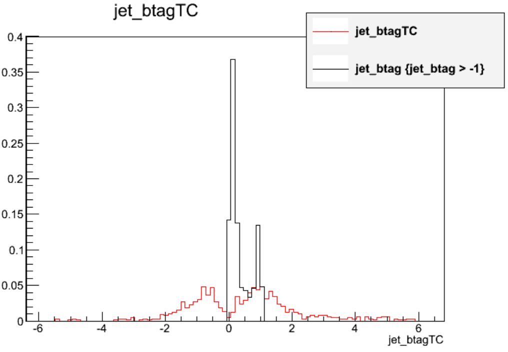
Let’s add the high purity track counting tagger, which was the most common tagger in 2011. After adding a new array declaration and branch in the top sections of PatJetAnalyzer.cc, we can call bDiscriminator() for these alternate tagger:

// Declarations
std::vector<double> jet_btag;
std::vector<double> jet_btagTC;

// Branches
mtree->Branch("jet_btag",&jet_btag);
mtree->Branch("jet_btagTC",&jet_btagTC);

// inside the jet loop
 jet_btag.push_back(itjet->bDiscriminator("combinedSecondaryVertexBJetTags"));
 jet_btag.push_back(itjet->bDiscriminator("trackCountingHighPurBJetTags"));

The distributions in ttbar events (excluding events with null values) look remarkably different! The CSV algorithm is a typical “multivariate” discriminant that ranges from 0 to 1 while the track counting discriminant represents a physics-based impact parameter quantity that has a much wider range of values. More information about the various taggers can be found here.

Exercise 2 option B: count medium CSV b tags

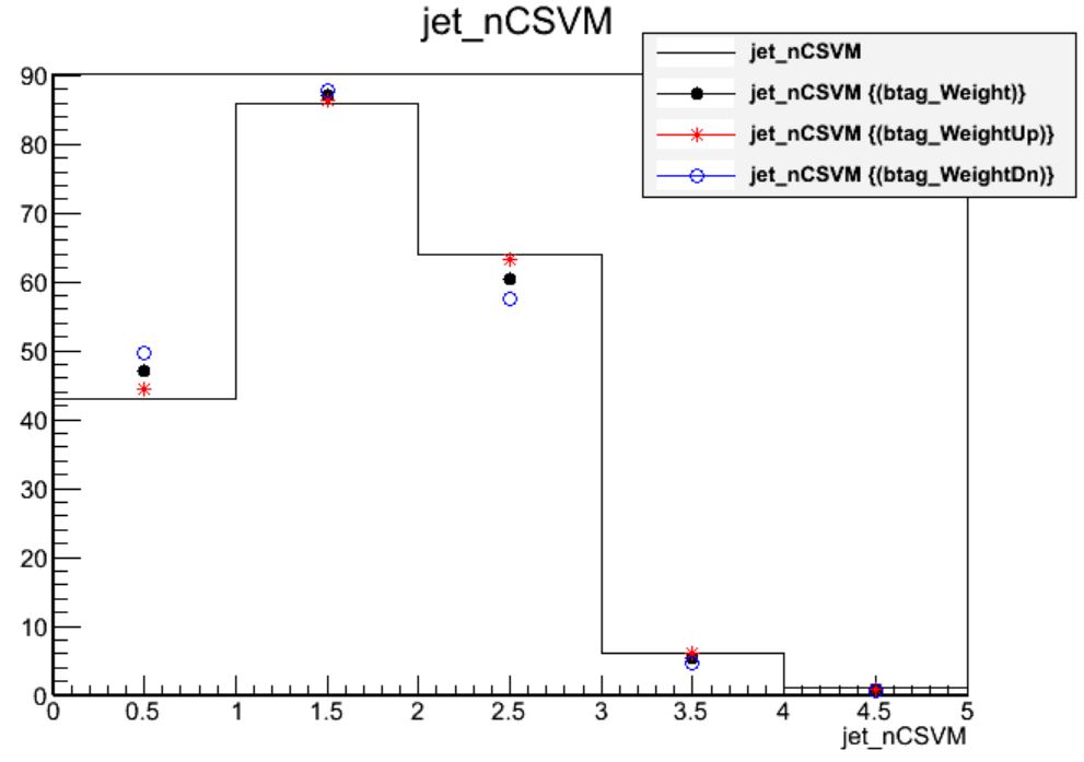
Calculate the number of jets per event that are b tagged according to the medium working point of the CSV algorithm. Store a branch called jet_nCSVM and draw it 3 times, applying the scale factor weights and demonstrating the uncertainty.

After editing PatJetAnalyzer.cc,

$ scram b
$ cmsRun python/poet_cfg.py False True
$ root -l myoutput.root
[0] _file0->cd("myjets")
[1] Events->Draw("jet_nCSVM","(btagWeight)")
[2] Events->Draw("jet_nCSVM","(btagWeightUp)","p hist same")
[3] Events->Draw("jet_nCSVM","(btagWeightDown)","p hist same")

Solution

We count the number of “Medium CSV” b-tagged jets by summing up the number of jets with discriminant values greater than 0.679. After adding a variable declaration and branch we can sum up the counter:

int jet_nCSVM = 0;
for (std::vector<pat::Jet>::const_iterator itjet=myjets->begin(); itjet!=myjets->end(); ++itjet){

 // ... JEC uncert, JER, storing variables...

 jet_btag.push_back(itjet->bDiscriminator("combinedSecondaryVertexBJetTags"));
 if (itjet->bDiscriminator("combinedSecondaryVertexBJetTags") > 0.679) jet_nCSVM++;
}

Applying the scale factor weight shifts the mean of the distribution down slightly. The uncertainty wraps around the central distribution with a magnitude of approximately 6% in this sample.

Key Points

• Muon corrections are a precision adjustment to a dimuon mass histogram.

• B tagging scale factors and uncertainties should be considered for any distribution that relies on b-tagged jets