Demo: Jet corrections
Overview
Teaching: 12 min
Exercises: 0 minQuestions
How are data/simulation differences dealt with for jet energy?
Objectives
Learn about typical differences in jet energy scale and resolution between data and simulation
Learn how JEC and JER corrections can be applied to OpenData jets
Access uncertainties in both JEC and JER
Unsurprisingly, the CMS detector does not measure jet energies perfectly, nor do simulation and data agree perfectly! The measured energy of jet must be corrected so that it can be related to the true energy of its parent particle. These corrections account for several effects and are factorized so that each effect can be studied independently. All of the corrections in this section are described in “Jet Energy Scale and Resolution” papers by CMS:
Correction levels
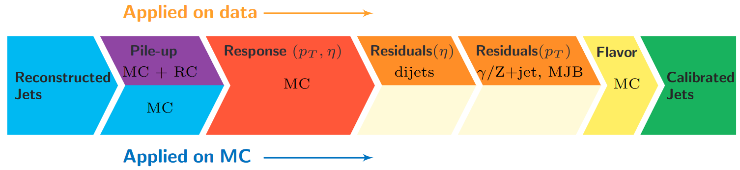
Particles from additional interactions in nearby bunch crossings of the LHC contribute energy in the calorimeters that must somehow be distinguished from the energy deposits of the main interaction. Extra energy in a jet’s cone can make its measured momentum larger than the momentum of the parent particle. The first layer (“L1”) of jet energy corrections accounts for pileup by subtracting the average transverse momentum contribution of the pileup interactions to the jet’s cone area. This average pileup contribution varies by pseudorapidity and, of course, by the number of interactions in the event.
The second and third layers of corrections (“L2L3”) correct the measured momentum to the true momentum as functions of momentum and pseudorapidity, bringing the reconstructed jet in line with the generated jet. These corrections are derived using momentum balancing and missing energy techniques in dijet and Z boson events. One well-measured object (ex: a jet near the center of the detector, a Z boson reconstructed from leptons) is balanced against a jet for which corrections are derived.
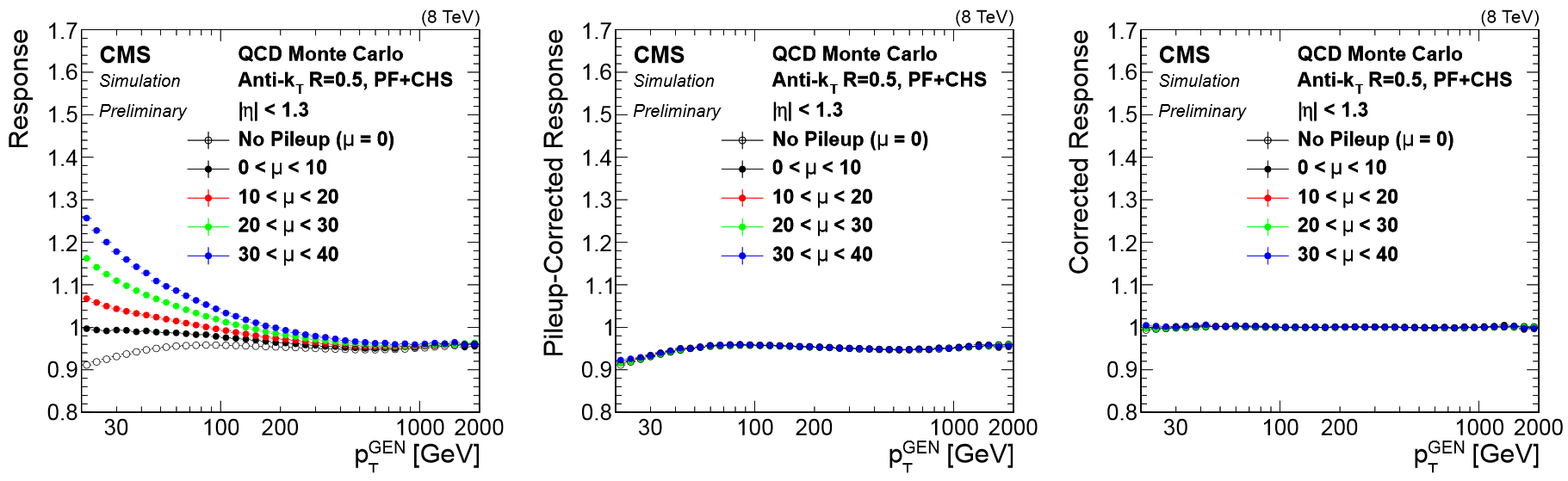
All of these corrections are applied to both data and simulation. Data events are then given “residual” corrections to bring data into line with the corrected simulation. A final set of flavor-based corrections are used in certain analyses that are especially sensitive to flavor effects. The figure below shows the result of the L1+L2+L3 corrections on the jet response.
Jet Energy Resolution
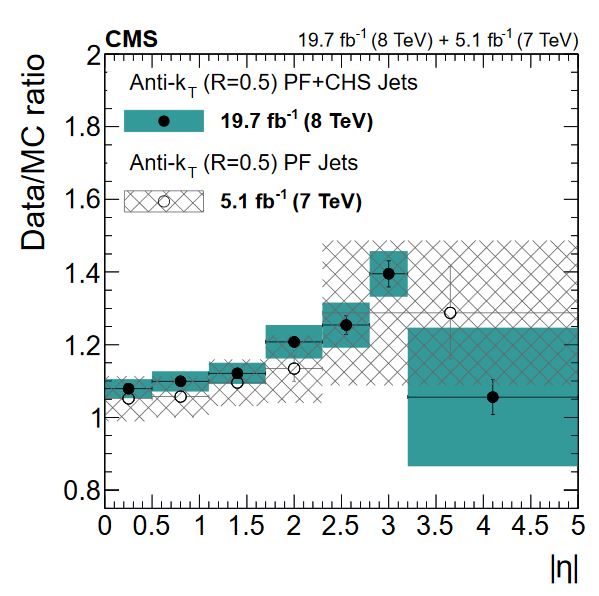
Jet Energy Resolution (JER) corrections are applied after JEC on strictly MC simulations. Unlike JEC, which adjusts the mean of the momentun response distribution, JER adjusts the width of the distribution. The ratio of reconstructed transverse momentum to true (generated) transverse momentum forms a Gaussian distributions – the width of this Gaussian is the JER. In data, where no “true” pT is available, the JER is measured using photon/Z + jet events where the jet recoils against the photon or Z boson, both of which can be measured quite precisely in the CMS detector. The JER is typically smaller in simulation than in data, leading to scale factors that are larger than 1. These scale factors, along with their uncertainties, are accessible in POET in the jet analyzers. They are applied using two methods:
- Adjusting the ratio of reconstructed to generated momentum using the scale factor (if a well-matched generated jet is found),
- Randomly smearing the momentum using a Gaussian distribution based on the resolution and scale factor (if no generated jet is found).
Applying JEC and JER
The jet energy corrections and Type-1 MET corrections can be applied to RECO jets while making PAT jets. To do this we will use the ‘addJetCollection’
process in python/poet_cfg.py. You can see that simulation and data use slightly different lists of correction levels as we discussed.
# Choose which jet correction levels to apply
jetcorrlabels = ['L1FastJet','L2Relative','L3Absolute']
if isData:
  # For data we need to remove generator-level matching processes
  runOnData(process, ['Jets','METs'], "", None, [])
  jetcorrlabels.append('L2L3Residual')

# Configure the addJetCollection tool
# This process will make corrected jets with b-tagging included, and will make Type1-corrected MET
process.ak5PFJets.doAreaFastjet = True
addJetCollection(process,cms.InputTag('ak5PFJets'),
    'AK5', 'PFCorr',
    doJTA        = True,
    doBTagging   = True,
    jetCorrLabel = ('AK5PF', cms.vstring(jetcorrlabels)),
    doType1MET   = True,
    doL1Cleaning = False,
    doL1Counters = False,
    doJetID      = True,
    jetIdLabel   = "ak5",
    )
In PatJetAnalyzer.cc the corrected momenta and energy come for free! For extra information we can access the uncorrected jet
and store some of its features as well.
for (std::vector<pat::Jet>::const_iterator itjet=myjets->begin(); itjet!=myjets->end(); ++itjet){
  pat::Jet uncorrJet = itjet->correctedJet(0);

  // itjet is the corrected jet and uncorrJet is the raw jet
}
The JER corrections must be accessed from a text file and applied on top of the corrected jets. The text file is
read in using the SimpleJetCorrector class which provides a correction() member function that will evaluate the formula
provided in the text file given the necessary variables (in this case: momentum, pseudorapidity, and number of pileup vertices).
In the constructor function PatJetAnalyzer::PatJetAnalyzer:
jerResName_ = iConfig.getParameter<edm::FileInPath>("jerResName").fullPath(); // JER Resolutions

JetCorrectorParameters *ak5PFPar = new JetCorrectorParameters(jerResName_);
jer_ = boost::shared_ptr<SimpleJetCorrector>( new SimpleJetCorrector(*ak5PFPar) );
We can now use jer_->correction() to access the jet’s momentum resolution in simulation. In the code snippet below you can see “scaling” and “smearing” versions of applying the JER scale factors, depending
on whether or not this pat::Jet had a matched generated jet. The random smearing application uses a reproducible seed for the random number generator based on the inherently random azimuthal angle of the jet.
Note: this code snippet is simplified by removing lines for handling uncertainties – that’s coming below!
for (std::vector<pat::Jet>::const_iterator itjet=myjets->begin(); itjet!=myjets->end(); ++itjet){
  pat::Jet uncorrJet = itjet->correctedJet(0);

  ptscale = 1;
  res = 1;
  if(!isData) {
    std::vector<float> factors = factorLookup(fabs(itjet->eta())); // returns in order {factor, factor_down, factor_up}
    std::vector<float> feta;
    std::vector<float> PTNPU;
    feta.push_back( fabs(itjet->eta()) );
    PTNPU.push_back( itjet->pt() );
    PTNPU.push_back( vertices->size() );

    res = jer_->correction(feta, PTNPU);

    float reco_pt = itjet->pt();
    const reco::GenJet *genJet = itjet->genJet();
    bool smeared = false;

    // Attempt the truth-vs-reco smearing
    if(genJet){
      double deltaPt = fabs(genJet->pt() - reco_pt);
      double deltaR = reco::deltaR(genJet->p4(),itjet->p4());
      if ((deltaR < 0.25) && deltaPt <= 2*reco_pt*res){
        double ptratio = reco_pt/genJet->pt();
        ptscale = max(0.0, ptratio + factors[0]*(1 - ptratio));
        smeared = true;
      }
    }
    // If that didn't work, use Gaussian smearing with a reproducible seed
    if (!smeared && factors[0] > 1) {
      TRandom3 JERrand;

      JERrand.SetSeed(abs(static_cast<int>(itjet->phi()*1e4)));
      ptscale = max(0.0, 1.0 + JERrand.Gaus(0,res)*sqrt(factors[0]*factors[0] - 1.0));
    }
  }
}
The final, definitive jet momentum is the raw momentum multiplied by both JEC and JER corrections! After computing ptscale, we store a variety of corrected and uncorrected kinematic variables for jets passing the momentum threshold:
if( ptscale*itjet->pt() <= min_pt) continue;

jet_pt.push_back(uncorrJet.pt());
// ...other variables...
corr_jet_pt.push_back(ptscale*itjet->pt());
Uncertainties
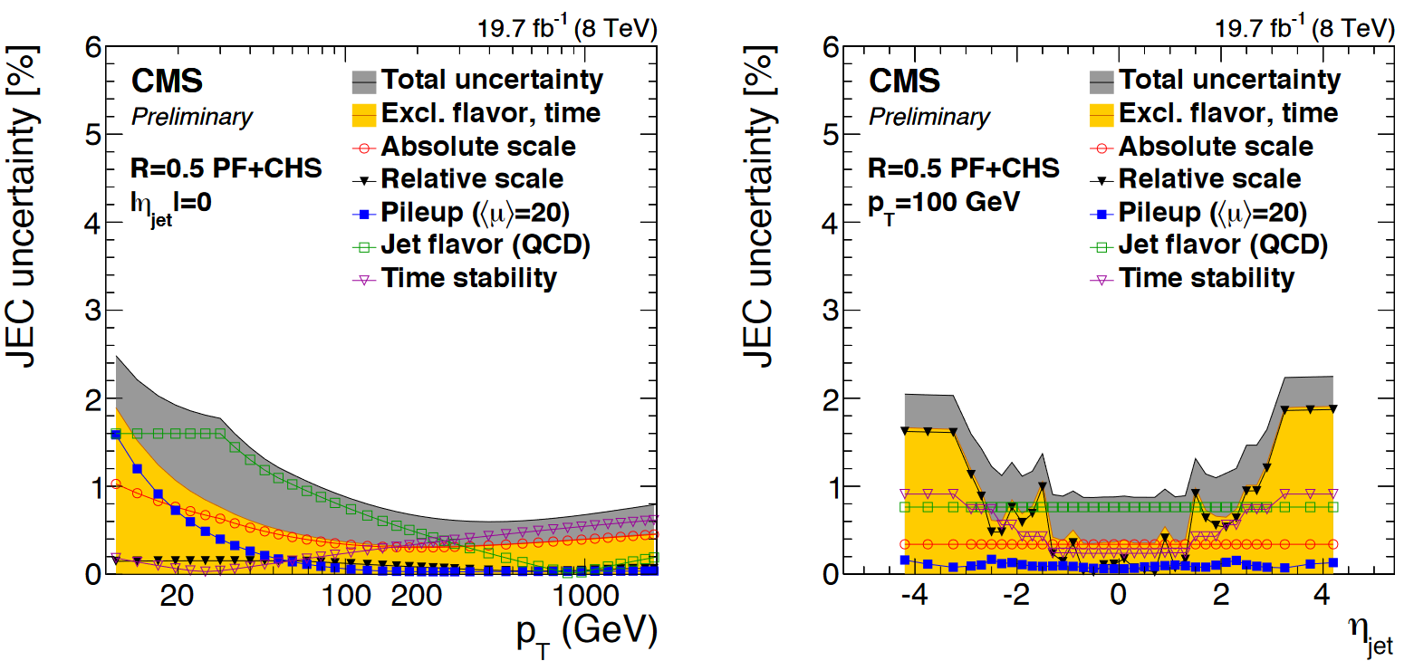
You will have noticed that nested among the JEC and JER code snippets given above were commands related to the uncertainty in these corrections. The JEC uncertainties have several sources, shown in the figure below. The L1 (pileup) uncertainty dominates at low momentum, while the L3 (absolute scale) uncertainty takes over for higher momentum jets. All corrections are quite precise for jets located near the center of the CMS barrel region, and the precision drops as pseudorapidity increases and different subdetectors lose coverage.
The JER uncertainty is evaluated by shifting the scale factors up and down according to the error bars shown in the scale factor figure above. These uncertainties arise from treatment of initial and final state radiation in the data measurement, differences in Monte Carlo tunes across generator platforms, and small non-Gaussian tail effects.
The JEC uncertainty text file is loaded as a JetCorrectionUncertainty object in the PatJetAnalyzer constructor:
jecUncName_ = iConfig.getParameter<edm::FileInPath>("jecUncName").fullPath(); // JEC uncertainties

jecUnc_ = boost::shared_ptr<JetCorrectionUncertainty>( new JetCorrectionUncertainty(jecUncName_) );
This object provides a getUncertainty() function that takes in the jet’s momentum and pseudorapidity and returns an adjustment to the JEC correction factor:
for (std::vector<pat::Jet>::const_iterator itjet=myjets->begin(); itjet!=myjets->end(); ++itjet){
  pat::Jet uncorrJet = itjet->correctedJet(0);

  double corrUp = 1.0;
  double corrDown = 1.0;
  jecUnc_->setJetEta( itjet->eta() );
  jecUnc_->setJetPt( itjet->pt() );
  corrUp = (1 + fabs(jecUnc_->getUncertainty(1)));
  jecUnc_->setJetEta( itjet->eta() );
  jecUnc_->setJetPt( itjet->pt() );
  corrDown = (1 - fabs(jecUnc_->getUncertainty(-1)));
The JER uncertainty is evaluated by calculating a ptscale_up and ptscale_down correction, exactly as shown above for the ptscale correction, but using the shifted scale factors. The uncertainties in JEC and JER are kept separate from each other: when varying JEC, the JER correction is held constant, and vice versa. This results in 5 momentum branches: a central value and two sets of uncertainties:
corr_jet_pt.push_back(ptscale*itjet->pt());
corr_jet_ptUp.push_back(ptscale*corrUp*itjet->pt());
corr_jet_ptDown.push_back(ptscale*corrDown*itjet->pt());
corr_jet_ptSmearUp.push_back(ptscale_up*itjet->pt());
corr_jet_ptSmearDown.push_back(ptscale_down*itjet->pt());
Key Points
Jet energy corrections are factorized and account for many mismeasurement effects
L1+L2+L3 should be applied to jets used for analyses, with residual corrections for data
Jet energy resolution in simulation is typically too narrow and is smeared using scale factors
Jet energy and resolution corrections are sources of systematic error and uncertainties should be evaluated