Heavy flavor tagging
Overview
Teaching: 10 min min
Exercises: 20 min minQuestions
How are b hadrons identified in CMS
Objectives
Understand the basics of heavy flavor tagging
Learn to access tagging information in AOD files
Jet reconstruction and identification is an important part of the analyses at the LHC. A jet may contain the hadronization products of any quark or gluon, or possibly the decay products of more massive particles such as W or Higgs bosons. Several “b tagging” algorithms exist to identify jets from the hadronization of b quarks, which have unique properties that distinguish them from light quark or gluon jets.
B Tagging Algorithms
Tagging algorithms first connect the jets with good quality tracks that are either associated with one of the jet’s particle flow candidates or within a nearby cone. Both tracks and “secondary vertices” (track vertices from the decays of b hadrons) can be used in track-based, vertex-based, or “combined” tagging algorithms. The specific details depend upon the algorithm use. However, they all exploit properties of b hadrons such as:
- long lifetime,
- large mass,
- high track multiplicity,
- large semileptonic branching fraction,
- hard fragmentation fuction.
Tagging algorithms are Algorithms that are used for b-tagging:
- Track Counting: identifies a b jet if it contains at least N tracks with significantly non-zero impact parameters.
- Jet Probability: combines information from all selected tracks in the jet and uses probability density functions to assign a probability to each track
- Soft Muon and Soft Electron: identifies b jets by searching for a lepton from a semi-leptonic b decay.
- Simple Secondary Vertex: reconstructs the b decay vertex and calculates a discriminator using related kinematic variables.
- Combined Secondary Vertex: exploits all known kinematic variables of the jets, information about track impact parameter significance and the secondary vertices to distinguish b jets. This tagger became the default CMS algorithm.
These algorithms produce a single, real number (often the output of an MVA) called a b tagging “discriminator” for each jet. The more positive the discriminator value, the more likely it is that this jet contained b hadrons.
Accessing tagging information
In AOD2NanoAOD.cc we access the information from the Combined Secondary Vertex (CSV) b tagging algorithm and associate discriminator values with the jets.
The CSV values are stored in a separate collection in the AOD files called a JetTagCollection, which is effectively a vector of associations between jet references and
float values (such as a b-tagging discriminator).
#include "DataFormats/JetReco/interface/PFJet.h"
#include "DataFormats/BTauReco/interface/JetTag.h"

Handle<PFJetCollection> jets;
iEvent.getByLabel(InputTag("ak5PFJets"), jets);

//define b-tag discriminators handle and get the discriminators
Handle<JetTagCollection> btags;
iEvent.getByLabel(InputTag("combinedSecondaryVertexBJetTags"), btags);

//loop over jets
const float jet_min_pt = 15;
value_jet_n = 0;
std::vector<PFJet> selectedJets;
for (auto it = jets->begin(); it != jets->end(); it++) {
  if (it->pt() > jet_min_pt) {

    // from the btag collection get the float (second) from the association to this jet.
    value_jet_btag[value_jet_n] = btags->operator[](it - jets->begin()).second;

  }
}
We can investigate at the b tag information in a dataset using ROOT.
$ root -l output.root
[0] _file0->cd("aod2nanoaod");
[1] Events->Draw("Jet_btag");
From the “Events” tree, select Jet_btag to see the distribution of discriminator values in the top quark pair file you processed earlier.
Challenge: alternate taggers
Use
edmDumpEventContentto investiate other b tagging algorithms available as edm::AssociationVector types. Add 1-2 new branches for alternate taggers and compare those discriminants to CSV (compile and run cmsRun as you’ve done before).Solution
Let’s add the MVA version of CSV and the high purity track counting tagger, which was the most common tagger in 2011. After adding new array declarations and branches in the top sections of
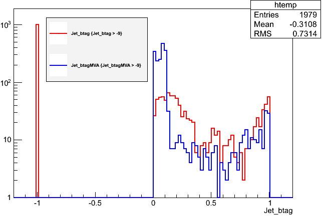
AOD2NanoAOD.cc, we can open the collections for these alternate taggers:Handle<JetTagCollection> btagsMVA, btagsTC; iEvent.getByLabel(InputTag("trackCountingHighPurBJetTags"), btagsTC); iEvent.getByLabel(InputTag("combinedSecondaryVertexMVABJetTags"), btagsMVA); // inside the jet loop value_jet_btagmva[value_jet_n] = btagsMVA->operator[](it - jets->begin()).second; value_jet_btagtc[value_jet_n] = btagsTC->operator[](it - jets->begin()).second;The distributions in ttbar events (excluding events with values of -9 where the tagger wasn’t evaluated) are shown below. The track counting discriminant is quite different and ranges 0 – 30 or so.
Working points
A jet is considered “b tagged” if the discriminator value exceeds some threshold. Different thresholds will have different efficiencies for identifying true b quark jets and for mis-tagging light quark jets. As we saw for muons and other objects, a “loose” working point will allow the highest mis-tagging rate, while a “tight” working point will sacrifice some correct-tag efficiency to reduce mis-tagging. The CSV algorithm has working points defined based on mis-tagging rate:
- Loose = ~10% mis-tagging = discriminator > 0.244
- Medium = ~1% mis-tagging = discriminator > 0.679
- Tight = ~0.1% mis-tagging = discriminator > 0.898
Challenge: count medium CSV b tags
Calculate the number of jets per event that are b tagged according to the medium working point of the CSV algorithm.
Solution
We count the number of “Medium CSV” b-tagged jets by summing up the number of jets with discriminant values greater than 0.679. After adding a variable declaration and branch we can sum up the counter:
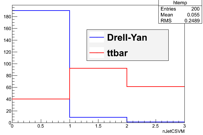
value_jet_nCSVM = 0;
for (auto it = jets->begin(); it != jets->end(); it++){

 // skipping bits

 value_jet_btag[value_jet_n] = btags->operator[](it - jets->begin()).second
 if (value_jet_btag[value_jet_n] > 0.679) value_jet_nCSVM++;
 value_jet_n++;
}
The distribution of the number of CSV b jets also shows a strong difference, as expected, between Drell-Yan and top pair events:
Data and simulation differences:
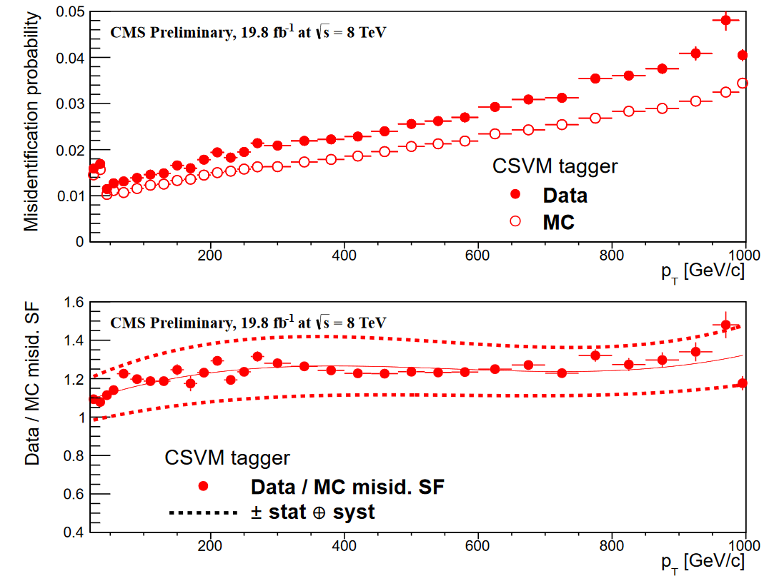
When training a tagging algorithm, it’s highly probable that the efficiencies for tagging different quark flavors as b jets will vary between simulation and data. These differences must be measured and corrected for using “scale factors” constructed from ratios of the efficiencies from different sources. The figures below show examples of the b and light quark efficiencies and scale factors as a function of jet momentum (read more).
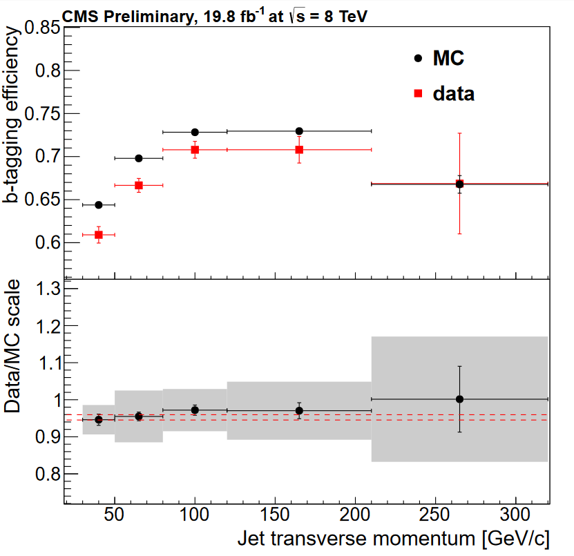
In simulation, the efficiency for tagging b quarks as b jets is defined as the number of “real b jets” (jets spatially matched to generator-level b hadrons)
tagged as b jets divided by the number of real b jets. The efficiency for mis-tagging c or light quarks as b jets is similar (real c/light jets tagged as b jets
/ real c/light jets). These values are typically computed as functions of the momentum or pseudorapidity of the jet. The “real” flavor of the jet is accessed most simply by creating pat::Jet objects instead of reco::Jet objects, as we will see in the next episode.
Scale factors to increase or decrease the number of b-tagged jets in simulation can be applied in a number of ways, but typically involve weighting simulation events based on the efficiencies and scale factors relevant to each jet in the event. Scale factors for the CSV algorithm are available for Open Data and involve extracting functions from a comma-separated-values file. Details and usage reference can be found here:
Watch for more efficiency and scale factor implementation examples in future updates to the Open Data Guide!
Key Points
Tagging algorithms separate heavy flavor jets from jets produced by the hadronization of light quarks and gluons
Tagging algorithms produce a disriminator value for each jet that represents the likelihood that the jet came from a b hadron
Each tagging algorithm has recommended ‘working points’ (discriminator values) based on a misidentification probability for light-flavor jets