CMS Jets and MET
Overview
Teaching: 10 min
Exercises: 15 minQuestions
How are jets and missing transverse energy accessed in CMS files?
Objectives
Identify jet and MET code collections in AOD files
Understand typical features of jet/MET objects
Practice accessing jet quantities
After tracks and energy deposits in the CMS tracking detectors (inner, muon) and calorimeters (electromagnetic, hadronic) are reconstructed as particle flow candidates, an event can be interpreted in various ways. Two common elements of event interpretation are clustering jets and calculating missing transverse momentum.
Jets
Jets are spatially-grouped collections of long-lived particles that are produced when a quark or gluon hadronizes. The kinetmatic properties of jets resemble that of the initial partons that produced them. In the CMS language, jets are made up of many particles, with the following predictable energy composition:
- ~65% charged hadrons
- ~25% photons (from neutral pions)
- ~10% neutral hadrons
Jets are very messy! Hadronization and the subsequent decays of unstable hadrons can produce 100s of particles near each other in the CMS detector. Hence these particles are rarely analyzed individually. How can we determine which particle candidates should be included in each jet?
Clustering
Jets can be clustered using a variety of different inputs from the CMS detector. “CaloJets” use only calorimeter energy deposits. “GenJets” use generated particles from a simulation. But by far the most common are “PFJets”, from particle flow candidates.
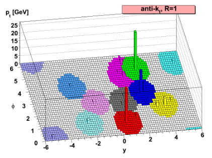
The result of the CMS Particle Flow algorithm is a list of particle candidates that account for all inner-tracker and muon tracks and all above-threshold energy deposits in the calorimeters. These particles are formed into jets using a “clustering algorithm”. The most common algorithm used by CMS is the “anti-kt” algorithm, which is abbreviated “AK”. It iterates over particle pairs and finds the two (i and j) that are the closest in some distance measure and determines whether to combine them:

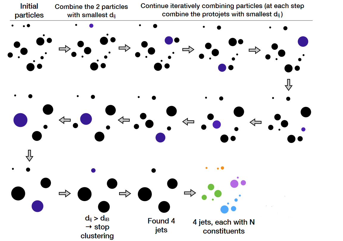
The momentum power (-2) used by the anti-kt algorithm means that higher-momentum particles are clustered first. This leads to jets with a round shape that tend to be centered on the hardest particle. In CMS software this clustering is implemented using the [[fastjet][www.fastjet.fr]] package.

Pileup
Inevitably, the list of particle flow candidates contains particles that did not originate from the primary interaction point. CMS experiences multiple simultaneous collisions, called “pileup”, during each “bunch crossing” of the LHC, so particles from multiple collisions coexist in the detector. There are various methods to remove their contributions from jets:
- Charged hadron subtraction CHS: all charged hadron candidates are associated with a track. If the track is not associated with the primary vertex, that charged hadron can be removed from the list. CHS is limited to the region of the detector covered by the inner tracker. The pileup contribution to neutral hadrons has to be removed mathematically – more in episode 3!
- PileUp Per Particle Identification (PUPPI, available in Run 2): CHS is applied, and then all remaining particles are weighted based on their likelihood of arising from pileup. This method is more stable and performant in high pileup scenarios such as the upcoming HL-LHC era.
Accessing jets in CMS software
Jets software classes have the same basic 4-vector methods as the objects discussed in the previous lesson:
Handle<CaloJetCollection> jets;
iEvent.getByLabel(InputTag("ak5PFJets"), jets);

for (auto it = jets->begin(); it != jets->end(); it++) {

    value_jet_pt[value_jet_n] = it->pt();
    value_jet_eta[value_jet_n] = it->eta();
    value_jet_phi[value_jet_n] = it->phi();
    value_jet_mass[value_jet_n] = it->mass();

}
Particle-flow jets are not immune to noise in the detector, and jets used in analyses should be filtered to remove noise jets. CMS has defined a Jet ID with criteria for good jets:
The PFlow jets are required to have charged hadron fraction CHF > 0.0 if within tracking fiducial region of |eta| < 2.4, neutral hadron fraction NHF < 1.0, charged electromagnetic (electron) fraction CEF < 1.0, and neutral electromagnetic (photon) fraction NEF < 1.0. These requirements remove fake jets arising from spurious energy depositions in a single sub-detector.
These criteria demonstrate how particle-flow jets combine information across subdetectors. Jets will typically have energy from electrons and photons, but those fractions of the total energy should be less than one. Similarly, jets should have some energy from charged hadrons if they overlap the inner tracker, and all the energy should not come from neutral hadrons. A mixture of energy sources is expected for genuine jets. All of these energy fractions (and more) can be accessed from the jet objects.
Challenge: Jet ID
Use the cms-sw github repository to learn the methods available for PFJets (hint: the header file is included from
AOD2NanoAOD.cc). Implement the jet ID and reject jets that do not pass. Rejection means that information about these jets will not be stored in any of the tree branches.Solution
The header file we need is for particle-flow jets:
interface/PFJet.hfrom the link given. It shows many functions like this:float chargedHadronEnergyFraction () const {return chargedHadronEnergy () / energy ();}These functions give the energy from a certain type of particle flow candidate as a fraction of the jet’s total energy. We can apply the conditions given to reject jets from noise at the same time we apply a momentum threshold:
for (auto it = jets->begin(); it != jets->end(); it++) {
 if (it->pt > jet_min_pt && it->chargedHadronEnergyFraction() > 0 && it->neutralHadronEnergyFraction() < 1.0 &&
     it->electronEnergyFraction() < 1.0 && it->photonEnergyFraction() < 1.0){

   // calculate things on jets
 }
}
MET
Missing transverse momentum is the negative vector sum of the transverse momenta of all particle flow candidates in an event. The magnitude of the missing transverse momentum vector is called missing transverse energy and referred to with the acronym “MET”. Since energy corrections are made to the particle flow jets, those corrections are propagated to MET by adding back the momentum vectors of the original jets and then subtracting the momentum vectors of the corrected jets. This correction is called “Type 1” and is standard for all CMS analyses. The jet energy corrections will be discussed more deeply at the end of this lesson.
In AOD2NanoAOD.cc we open the particle flow MET module and extract the magnitude and angle of the MET, the sum of all energy
in the detector, and variables related to the “significance” of the MET. Note that MET quantities have a single value for the
entire event, unlike the objects studied previously.
Handle<PFMETCollection> met;
iEvent.getByLabel(InputTag("pfMet"), met);

value_met_pt = met->begin()->pt();
value_met_phi = met->begin()->phi();
value_met_sumet = met->begin()->sumEt();

value_met_significance = met->begin()->significance();
auto cov = met->begin()->getSignificanceMatrix();
value_met_covxx = cov[0][0];
value_met_covxy = cov[0][1];
value_met_covyy = cov[1][1];
MET significance can be a useful tool: it describes the likelihood that the MET arose from noise or mismeasurement in the detector as opposed to a neutrino or similar non-interacting particle. The four-vectors of the other physics objects along with their uncertainties are required to compute the significance of the MET signature. MET that is directed nearly (anti)colinnear with a physics object is likely to arise from mismeasurement and should not have a large significance.
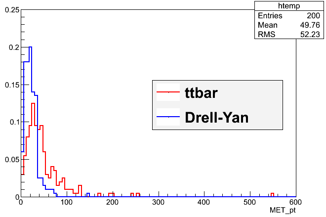
Challenge: real and fake MET
Compile all your changes to
AOD2NanoAOD.ccso far and run over the simulation sample again. This test file contains top quark pair events, so some events will have leptonic decays that include neutrinos and some events will not. Review TTree::Draw from the pre-exercises – can you draw histograms of MET versus MET significance and infer which events have leptonic decays?$ scram b $ cmsRun configs/simulation_cfg.py $ # edit simulation_cfg.py to use the Drell-Yan test file, and save output_DY.root $ cmsRun confings/simulation_cfg.py $ root -l output.root [0] TTree *ttbar = (TTree*)_file0->Get("aod2nanoaod/Events"); [1] TFile *_file1 = TFile::Open("output_DY.root"); [2] TTree *dy = (TTree*)_file1->Get("aod2nanoaod/Events"); [3] ttbar->Draw("...things...","...any cuts...","norm) [4] dy->Draw("...things...","...any cuts...","norm pe same")Solution
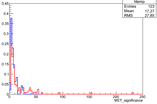
The difference between the Drell-Yan events with primarily fake MET and the top pair events with primarily genuine MET can be seen by drawing
MET_ptor by drawingMET_significance. In both distributions the Drell-Yan events have smaller values than the top pair events.
Key Points
Jets are spatially-grouped collections of particles that traversed the CMS detector
Particles from additional proton-proton collisions (pileup) must be removed from jets
Missing transverse energy is the negative vector sum of particle candidates
Many of the class methods discussed for other objects can be used for jets
Heavy flavor tagging
Overview
Teaching: 10 min min
Exercises: 20 min minQuestions
How are b hadrons identified in CMS
Objectives
Understand the basics of heavy flavor tagging
Learn to access tagging information in AOD files
Jet reconstruction and identification is an important part of the analyses at the LHC. A jet may contain the hadronization products of any quark or gluon, or possibly the decay products of more massive particles such as W or Higgs bosons. Several “b tagging” algorithms exist to identify jets from the hadronization of b quarks, which have unique properties that distinguish them from light quark or gluon jets.
B Tagging Algorithms
Tagging algorithms first connect the jets with good quality tracks that are either associated with one of the jet’s particle flow candidates or within a nearby cone. Both tracks and “secondary vertices” (track vertices from the decays of b hadrons) can be used in track-based, vertex-based, or “combined” tagging algorithms. The specific details depend upon the algorithm use. However, they all exploit properties of b hadrons such as:
- long lifetime,
- large mass,
- high track multiplicity,
- large semileptonic branching fraction,
- hard fragmentation fuction.
Tagging algorithms are Algorithms that are used for b-tagging:
- Track Counting: identifies a b jet if it contains at least N tracks with significantly non-zero impact parameters.
- Jet Probability: combines information from all selected tracks in the jet and uses probability density functions to assign a probability to each track
- Soft Muon and Soft Electron: identifies b jets by searching for a lepton from a semi-leptonic b decay.
- Simple Secondary Vertex: reconstructs the b decay vertex and calculates a discriminator using related kinematic variables.
- Combined Secondary Vertex: exploits all known kinematic variables of the jets, information about track impact parameter significance and the secondary vertices to distinguish b jets. This tagger became the default CMS algorithm.
These algorithms produce a single, real number (often the output of an MVA) called a b tagging “discriminator” for each jet. The more positive the discriminator value, the more likely it is that this jet contained b hadrons.
Accessing tagging information
In AOD2NanoAOD.cc we access the information from the Combined Secondary Vertex (CSV) b tagging algorithm and associate discriminator values with the jets.
The CSV values are stored in a separate collection in the AOD files called a JetTagCollection, which is effectively a vector of associations between jet references and
float values (such as a b-tagging discriminator).
#include "DataFormats/JetReco/interface/PFJet.h"
#include "DataFormats/BTauReco/interface/JetTag.h"

Handle<PFJetCollection> jets;
iEvent.getByLabel(InputTag("ak5PFJets"), jets);

//define b-tag discriminators handle and get the discriminators
Handle<JetTagCollection> btags;
iEvent.getByLabel(InputTag("combinedSecondaryVertexBJetTags"), btags);

//loop over jets
const float jet_min_pt = 15;
value_jet_n = 0;
std::vector<PFJet> selectedJets;
for (auto it = jets->begin(); it != jets->end(); it++) {
  if (it->pt() > jet_min_pt) {

    // from the btag collection get the float (second) from the association to this jet.
    value_jet_btag[value_jet_n] = btags->operator[](it - jets->begin()).second;

  }
}
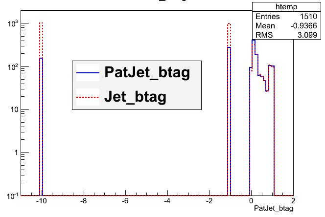
We can investigate at the b tag information in a dataset using ROOT.
$ root -l output.root
[0] _file0->cd("aod2nanoaod");
[1] Events->Draw("Jet_btag");
From the “Events” tree, select Jet_btag to see the distribution of discriminator values in the top quark pair file you processed earlier.
Challenge: alternate taggers
Use
edmDumpEventContentto investiate other b tagging algorithms available as edm::AssociationVector types. Add 1-2 new branches for alternate taggers and compare those discriminants to CSV (compile and run cmsRun as you’ve done before).Solution
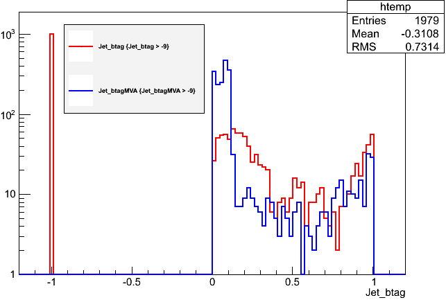
Let’s add the MVA version of CSV and the high purity track counting tagger, which was the most common tagger in 2011. After adding new array declarations and branches in the top sections of
AOD2NanoAOD.cc, we can open the collections for these alternate taggers:Handle<JetTagCollection> btagsMVA, btagsTC; iEvent.getByLabel(InputTag("trackCountingHighPurBJetTags"), btagsTC); iEvent.getByLabel(InputTag("combinedSecondaryVertexMVABJetTags"), btagsMVA); // inside the jet loop value_jet_btagmva[value_jet_n] = btagsMVA->operator[](it - jets->begin()).second; value_jet_btagtc[value_jet_n] = btagsTC->operator[](it - jets->begin()).second;The distributions in ttbar events (excluding events with values of -9 where the tagger wasn’t evaluated) are shown below. The track counting discriminant is quite different and ranges 0 – 30 or so.
Working points
A jet is considered “b tagged” if the discriminator value exceeds some threshold. Different thresholds will have different efficiencies for identifying true b quark jets and for mis-tagging light quark jets. As we saw for muons and other objects, a “loose” working point will allow the highest mis-tagging rate, while a “tight” working point will sacrifice some correct-tag efficiency to reduce mis-tagging. The CSV algorithm has working points defined based on mis-tagging rate:
- Loose = ~10% mis-tagging = discriminator > 0.244
- Medium = ~1% mis-tagging = discriminator > 0.679
- Tight = ~0.1% mis-tagging = discriminator > 0.898
Challenge: count medium CSV b tags
Calculate the number of jets per event that are b tagged according to the medium working point of the CSV algorithm.
Solution
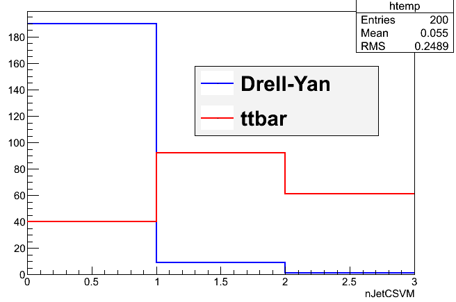
We count the number of “Medium CSV” b-tagged jets by summing up the number of jets with discriminant values greater than 0.679. After adding a variable declaration and branch we can sum up the counter:
value_jet_nCSVM = 0;
for (auto it = jets->begin(); it != jets->end(); it++){

 // skipping bits

 value_jet_btag[value_jet_n] = btags->operator[](it - jets->begin()).second
 if (value_jet_btag[value_jet_n] > 0.679) value_jet_nCSVM++;
 value_jet_n++;
}
The distribution of the number of CSV b jets also shows a strong difference, as expected, between Drell-Yan and top pair events:
Data and simulation differences:
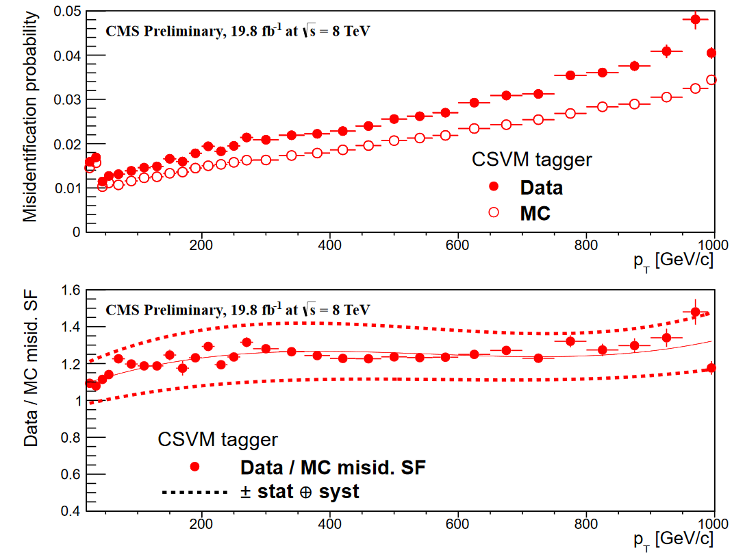
When training a tagging algorithm, it’s highly probable that the efficiencies for tagging different quark flavors as b jets will vary between simulation and data. These differences must be measured and corrected for using “scale factors” constructed from ratios of the efficiencies from different sources. The figures below show examples of the b and light quark efficiencies and scale factors as a function of jet momentum (read more).
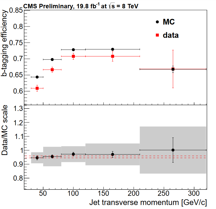
In simulation, the efficiency for tagging b quarks as b jets is defined as the number of “real b jets” (jets spatially matched to generator-level b hadrons)
tagged as b jets divided by the number of real b jets. The efficiency for mis-tagging c or light quarks as b jets is similar (real c/light jets tagged as b jets
/ real c/light jets). These values are typically computed as functions of the momentum or pseudorapidity of the jet. The “real” flavor of the jet is accessed most simply by creating pat::Jet objects instead of reco::Jet objects, as we will see in the next episode.
Scale factors to increase or decrease the number of b-tagged jets in simulation can be applied in a number of ways, but typically involve weighting simulation events based on the efficiencies and scale factors relevant to each jet in the event. Scale factors for the CSV algorithm are available for Open Data and involve extracting functions from a comma-separated-values file. Details and usage reference can be found here:
Watch for more efficiency and scale factor implementation examples in future updates to the Open Data Guide!
Key Points
Tagging algorithms separate heavy flavor jets from jets produced by the hadronization of light quarks and gluons
Tagging algorithms produce a disriminator value for each jet that represents the likelihood that the jet came from a b hadron
Each tagging algorithm has recommended ‘working points’ (discriminator values) based on a misidentification probability for light-flavor jets
Jet corrections
Overview
Teaching: 15 min
Exercises: 20 minQuestions
How are data/simulation differences dealt with for jets and MET?
Objectives
Learn about typical differences in jet energy scale and resolution between data and simulation
Understand how these corrections are applied to jets and MET
Access the uncertainties in the jet energy correction
Practice saving jet observables with uncertainties
Unsurprisingly, the CMS detector does not measure jet energies perfectly, nor do simulation and data agree perfectly! The measured energy of jet must be corrected so that it can be related to the true energy of its parent particle. These corrections account for several effects and are factorized so that each effect can be studied independently.
Correction levels
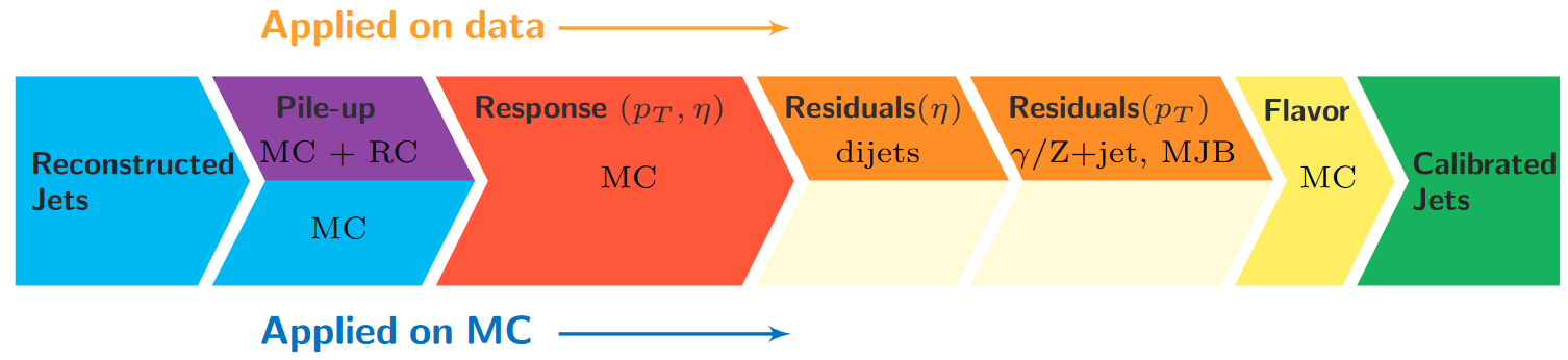
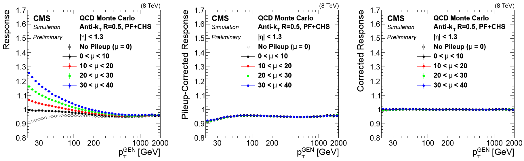
Particles from additional interactions in nearby bunch crossings of the LHC contribute energy in the calorimeters that must somehow be distinguished from the energy deposits of the main interaction. Extra energy in a jet’s cone can make its measured momentum larger than the momentum of the parent particle. The first layer (“L1”) of jet energy corrections accounts for pileup by subtracting the average transverse momentum contribution of the pileup interactions to the jet’s cone area. This average pileup contribution varies by pseudorapidity and, of course, by the number of interactions in the event.
The second and third layers of corrections (“L2L3”) correct the measured momentum to the true momentum as functions of momentum and pseudorapidity, bringing the reconstructed jet in line with the generated jet. These corrections are derived using momentum balancing and missing energy techniques in dijet and Z boson events. One well-measured object (ex: a jet near the center of the detector, a Z boson reconstructed from leptons) is balanced against a jet for which corrections are derived.
All of these corrections are applied to both data and simulation. Data events are then given “residual” corrections to bring data into line with the corrected simulation. A final set of flavor-based corrections are used in certain analyses that are especially sensitive to flavor effects. All of the corrections are described in this paper. The figure below shows the result of the L1+L2+L3 corrections on the jet response.
JEC from text files
There are several methods available for applying jet energy corrections to reconstructed jets. We have demonstrated a method to read in the corrections from text files and extract the corrections manually for each jet. The text files can be extracted from the global tag. First, set up sym links to the conditions databases for 2012 data and simulation (reference instructions):
Link database files
You might have done this in the pre-exercises! But if not, do it now. You will also need CVMFS mounted in your VM or docker container, which is covered in the pre-exercises.
$ ln -sf /cvmfs/cms-opendata-conddb.cern.ch/FT53_V21A_AN6_FULL FT53_V21A_AN6
$ ln -sf /cvmfs/cms-opendata-conddb.cern.ch/FT53_V21A_AN6_FULL.db FT53_V21A_AN6_FULL.db
$ ln -sf /cvmfs/cms-opendata-conddb.cern.ch/FT53_V21A_AN6_FULL FT53_V21A_AN6_FULL
$ ln -sf /cvmfs/cms-opendata-conddb.cern.ch/START53_V27 START53_V27
$ ln -sf /cvmfs/cms-opendata-conddb.cern.ch/START53_V27.db START53_V27.db
$ ls -l   ## make sure you see the full links as written above
To write out text files, we will use configs/jec_cfg.py, which uses a small analyzer to open the database files we just linked:
# connect to global tag
if isData:
    process.GlobalTag.connect = cms.string('sqlite_file:/cvmfs/cms-opendata-conddb.cern.ch/FT53_V21A_AN6_FULL.db')
    process.GlobalTag.globaltag = 'FT53_V21A_AN6::All'
else:
    process.GlobalTag.connect = cms.string('sqlite_file:/cvmfs/cms-opendata-conddb.cern.ch/START53_V27.db')
    process.GlobalTag.globaltag = 'START53_V27::All'


# setup JetCorrectorDBReader
process.maxEvents = cms.untracked.PSet(input=cms.untracked.int32(1))
process.source = cms.Source('EmptySource')
process.ak5 = cms.EDAnalyzer('JetCorrectorDBReader',
                             payloadName=cms.untracked.string('AK5PF'),
                             printScreen=cms.untracked.bool(False),
                             createTextFile=cms.untracked.bool(True))

if isData:
    process.ak5.globalTag = cms.untracked.string('FT53_V21A_AN6')
else:
    process.ak5.globalTag = cms.untracked.string('START53_V27')
Make the text files
Run this job once with
isData = Trueand once withisData = False(if you access the condition database for the first time, this will take a while). Then move the text files to thedata/directory:$ cmsRun configs/jec_cfg.py $ ## edit the file and flip isData $ cmsRun configs/jec_cfg.py $ mv *AK5PF.txt data/
In simulation_cfg.py the file names are passed to the AOD2NanoAOD analyzer:
process.aod2nanoaod = cms.EDAnalyzer("AOD2NanoAOD",
        jecL1Name = cms.FileInPath('workspace/AOD2NanoAODOutreachTool/data/START53_V27_L1FastJet_AK5PF.txt'),
        jecL2Name = cms.FileInPath('workspace/AOD2NanoAODOutreachTool/data/START53_V27_L2Relative_AK5PF.txt'),
        jecL3Name = cms.FileInPath('workspace/AOD2NanoAODOutreachTool/data/START53_V27_L3Absolute_AK5PF.txt'),
        jecUncName = cms.FileInPath('workspace/AOD2NanoAODOutreachTool/data/START53_V27_Uncertainty_AK5PF.txt'),
        isData = cms.bool(False)
In AOD2NanoAOD.cc the files are read to build a factorizedJetCorrector object from which the corrections can be accessed:
// Object definitions
bool isData;
std::vector<std::string> jecPayloadNames_;
std::string              jecL1_;
std::string              jecL2_;
std::string              jecL3_;
boost::shared_ptr<FactorizedJetCorrector> jec_;

// In the constructor the factorizedJetCorrected is set up
AOD2NanoAOD::AOD2NanoAOD(const edm::ParameterSet &iConfig){
  isData = iConfig.getParameter<bool>("isData");
  jecL1_ = iConfig.getParameter<edm::FileInPath>("jecL1Name").fullPath(); // JEC level payloads
  jecL2_ = iConfig.getParameter<edm::FileInPath>("jecL2Name").fullPath(); // JEC level payloads
  jecL3_ = iConfig.getParameter<edm::FileInPath>("jecL3Name").fullPath(); // JEC level payloads

  //Get the factorized jet corrector parameters.
  jecPayloadNames_.push_back(jecL1_);
  jecPayloadNames_.push_back(jecL2_);
  jecPayloadNames_.push_back(jecL3_);

  std::vector<JetCorrectorParameters> vPar;
  for ( std::vector<std::string>::const_iterator payloadBegin = jecPayloadNames_.begin(),
    payloadEnd = jecPayloadNames_.end(), ipayload = payloadBegin; ipayload != payloadEnd; ++ipayload ) {
    JetCorrectorParameters pars(*ipayload);
    vPar.push_back(pars);
    }

  // Make the FactorizedJetCorrector and Uncertainty
  jec_ = boost::shared_ptr<FactorizedJetCorrector> ( new FactorizedJetCorrector(vPar) );

  // ....function continues
}
In the analyze function the correction is evaluated for each jet. The correction depends on
the momentum, pseudorapidity, energy, and cone area of the jet, as well as the value of “rho” (the average momentum
per area) and number of interactions in the event. The correction is used to scale the momentum of the jet.
Handle<double> rhoHandle;
iEvent.getByLabel(InputTag("fixedGridRhoFastjetAll"), rhoHandle);

for (auto it = jets->begin(); it != jets->end(); it++) {
  if (it->pt() > jet_min_pt) {

    reco::Candidate::LorentzVector uncorrJet = it->p4();
    jec_->setJetEta( uncorrJet.eta() );
    jec_->setJetPt ( uncorrJet.pt() );
    jec_->setJetE  ( uncorrJet.energy() );
    jec_->setJetA  ( it->jetArea() );
    jec_->setRho   ( *(rhoHandle.product()) );
    jec_->setNPV   ( vertices->size() );

    double corr = jec_->getCorrection();

    value_jet_pt[value_jet_n] = it->pt();
    value_corr_jet_pt[value_jet_n] = corr * uncorrJet.pt();

  }
}
Challenge: add L2L3 residual corrections to data
In data, the L2L3 residual corrections should also be applied. Use the “isData” switch and set up
AOD2NanoAOD.ccanddata_cfg.pyto fully correct jets in data.Solution
When processing data, we need to open 4 text files rather than 3. This happens first in the config, which is actually missing ALL the text files right now! No switching is needed since we have a separate data config, but python if statements can be used if you want to have one configuration file for both data and simulation (left as an exercise to the reader). The text files for data start with “FT53” rather than “START53”:
process.aod2nanoaod = cms.EDAnalyzer("AOD2NanoAOD",
		      isData = cms.bool(True),
		      doPat = cms.bool(False),
		      jecL1Name = cms.FileInPath('workspace/AOD2NanoAODOutreachTool/data/FT53_V21A_AN6_L1FastJet_AK5PF.txt')
		      jecL2Name = cms.FileInPath('workspace/AOD2NanoAODOutreachTool/data/FT53_V21A_AN6_L2Relative_AK5PF.txt')
		      jecL3Name = cms.FileInPath('workspace/AOD2NanoAODOutreachTool/data/FT53_V21A_AN6_L3Absolute_AK5PF.txt')
		      jecResName = cms.FileInPath('workspace/AOD2NanoAODOutreachTool/data/FT53_V21A_AN6_L2L3Residual_AK5PF.txt')
		      jecUncName = cms.FileInPath('workspace/AOD2NanoAODOutreachTool/data/FT53_V21A_AN6_Uncertainty_AK5PF.txt')
		      )
In the source code we need to: teach the code about L2L3Residual, open that file only is
isData, and apply uncertainties only if!isData. The first task is done in the class definition:std::string jecL3_; std::string jecRes_;The second task is done in the constructor function of
AOD2NanoAOD:jecL3_ = iConfig.getParameter<edm::FileInPath>("jecL3Name").fullPath(); jecRes_ = iConfig.getParameter<edm::FileInPath>("jecResName").fullPath(); jecPayloadNames_.push_back(jecL3_); if(isData) jecPayloadNames_.push_back(jecRes_);And finally, we should escape the uncertainty calculation (more info on this below!) in the jet loop if we are working on data:
 double corrUp = 1.0;
 double corrDown = 1.0;
 if(!isData){
   jecUnc_->setJetEta( uncorrJet.eta() );
   // etc, through accessing corrUp and corrDown
 }
Jet Energy Resolution
These corrections account for differences between the true and measured energy scale of jets, but not the energy resolution. The jet momentum resolution is typically too small in simulation and is widened using a Gaussian smearing technique. Watch for implementation details on this correction in a future update to the Open Data Guide.
JEC while producing pat::Jets
Another popular object format in CMS is the “Physics Analysis Toolkit” format, called PAT. The jet energy corrections and Type-1 MET corrections can be
applied to RECO jets while making PAT jets. To do this we will load the global tag and databases directly in the configuration file and use the ‘addJetCollection’
process to create a collection of pat::jets. Look at simulation_patjets_cfg.py:
# Set up the new jet collection
process.ak5PFJets.doAreaFastjet = True
addPfMET(process, 'PF')

addJetCollection(process,cms.InputTag('ak5PFJets'),
                 'AK5', 'PFCorr',
                 doJTA        = True,
                 doBTagging   = True,
                 jetCorrLabel = ('AK5PF', cms.vstring(['L1FastJet','L2Relative','L3Absolute']))
                 doType1MET   = True,
                 doL1Cleaning = True,
                 doL1Counters = False,
                 doJetID      = True,
                 jetIdLabel   = "ak5",
                 )
In AOD2NanoAOD.cc we can look at the sections marked if(doPat) to see the difference in usage. In general, pat::jets are more
complex to create in the configuration file, but simpler to use because of their additional functions. In particular, accessing the
jet’s flavor directly makes calculation of b-tagging efficiencies and scale factors simpler.
  if(doPat){

    Handle<PFMETCollection> metT1;
    iEvent.getByLabel(InputTag("pfType1CorrectedMet"), metT1);
    value_met_type1_pt = metT1->begin()->pt();

    Handle<std::vector<pat::Jet> > patjets;
    iEvent.getByLabel(InputTag("selectedPatJetsAK5PFCorr"), patjets);

    value_patjet_n = 0;
    for (auto it = patjets->begin(); it != patjets->end(); it++) {
      if (it->pt() > jet_min_pt) {

        // Corrected values are now the default
        value_patjet_pt[value_patjet_n] = it->pt();
        value_patjet_eta[value_patjet_n] = it->eta();
        value_patjet_mass[value_patjet_n] = it->mass();

        // but uncorrected values can be accessed. JetID should be computed from the uncorrected jet
        pat::Jet uncorrJet = it->correctedJet(0);
        value_uncorr_patjet_pt[value_patjet_n] = uncorrJet.pt();
        value_uncorr_patjet_eta[value_patjet_n] = uncorrJet.eta();
        value_uncorr_patjet_mass[value_patjet_n] = uncorrJet.mass();

        // b-tagging is built in. Can access the truth flavor needed for b-tag effs & scale factor application!
        value_patjet_hflav[value_patjet_n] = it->hadronFlavour();
        value_patjet_btag[value_patjet_n] = it->bDiscriminator( "pfCombinedSecondaryVertexBJetTags");

        value_patjet_n++;
      }
    }
  }
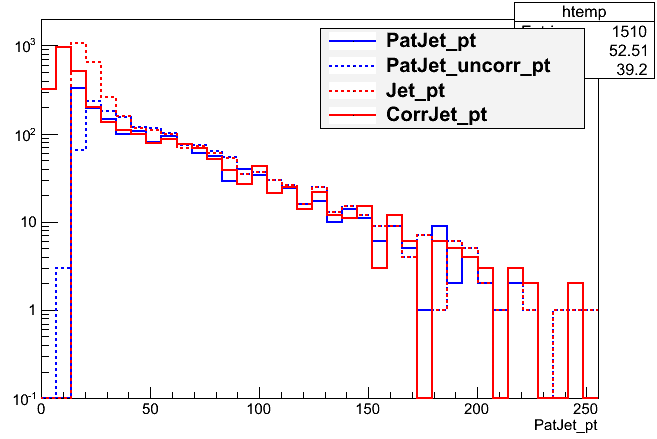
Challenge: create PAT jets
Run
simulation_patjets_cfg.py, open the file, and compare the two jet correction and b-tagging methods. Method 1 hasJet_andCorrJet_branches and Method 2 hasPatJet_andPatJet_uncorrbranches.Solution
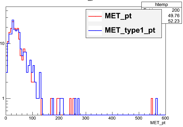
We can clearly see the difference between corrected and uncorrected jet momentum, particularly at low momentum where the effects of pileup are largest as a fraction of the total jet energy. here are differences in the number of jets across the collections because of different applications of the pt threshold (applied to uncorrected PFJets and corrected PATJets). We can also see small differences between particle-flow MET and type-1 corrected MET. The b-tagging distribution is almost identical, with the majority of the differences between the jet collections lying in the “dummy” value columns.
Uncertainties
You will have noticed that nested among the jet energy correction code snippets give above were commands related to the uncertainty in this correction. The uncertainty is also read from a text file in this example, and is used to increase or decrease the correction to the jet momentum.
// Object definition
boost::shared_ptr<FactorizedJetCorrector> jec_;

// In the constructor the JetCorrectionUncertainty is set up
AOD2NanoAOD::AOD2NanoAOD(const edm::ParameterSet &iConfig){

  jecUncName_ = iConfig.getParameter<edm::FileInPath>("jecUncName").fullPath();      // JEC uncertainties
  jecUnc_ = boost::shared_ptr<JetCorrectionUncertainty>( new JetCorrectionUncertainty(jecUncName_) );

  // ....function continues
}

// In the analyze function the uncertainty is evaluated
for (auto it = jets->begin(); it != jets->end(); it++) {
  if (it->pt() > jet_min_pt) {

    double corr = jec_->getCorrection();

    jecUnc_->setJetEta( uncorrJet.eta() );
    jecUnc_->setJetPt( corr * uncorrJet.pt() );
    double corrUp = corr * (1 + fabs(jecUnc_->getUncertainty(1)));
    double corrDown = corr * ( 1 - fabs(jecUnc_->getUncertainty(-1)) );

    value_corr_jet_ptUp[value_jet_n] = corrUp * uncorrJet.pt();
    value_corr_jet_ptDown[value_jet_n] = corrDown * uncorrJet.pt();

  }
}
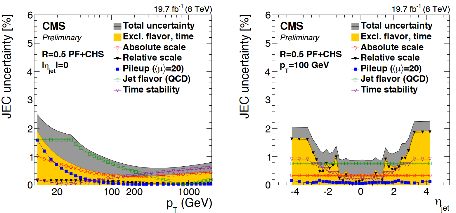
The uncertainties have several sources, shown in the figure below. The L1 (pileup) uncertainty dominates at low momentum, while the L3 (absolute scale) uncertainty takes over for higher momentum jets. All corrections are quite precise for jets located near the center of the CMS barrel region, and the precision drops as pseudorapidity increases and different subdetectors lose coverage.
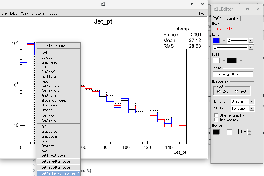
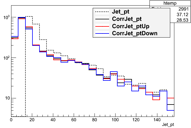
Challenge: shifted histograms
Plot and investigate the range of momentum variation given by the JEC uncertainties. Is the difference between the raw and corrected momentum larger or smaller than the uncertainty? Use TTree::Draw to make histograms of the various momentum distributions. Ideally, show the up and down variations in different colors, and the raw vs corrected momenta with different line styles.
Solution
Draw a histogram, hover over one of the lines, and right click. You should see a menu appear – select “Set Line Attributes” and a GUI with pop up. This is handy for changing line colors and styles interactively. Over the bulk of the momentum distribution, the jet energy corrections are significant – the corrected and uncorrected versions are not consistent within the uncertainty. Drawing these plots is a typical sanity check in CMS analyses to test whether the uncertainties look sensible.
Key Points
Jet energy corrections are factorized and account for many mismeasurement effects
L1+L2+L3 should be applied to jets used for analyses, with residual corrections for data
Jet energy corrections are an source of systematic error and uncertainties should be evaluated