Jet corrections
Overview
Teaching: 15 min
Exercises: 20 minQuestions
How are data/simulation differences dealt with for jets and MET?
Objectives
Learn about typical differences in jet energy scale and resolution between data and simulation
Understand how these corrections are applied to jets and MET
Access the uncertainties in the jet energy correction
Practice saving jet observables with uncertainties
Unsurprisingly, the CMS detector does not measure jet energies perfectly, nor do simulation and data agree perfectly! The measured energy of jet must be corrected so that it can be related to the true energy of its parent particle. These corrections account for several effects and are factorized so that each effect can be studied independently.
Correction levels
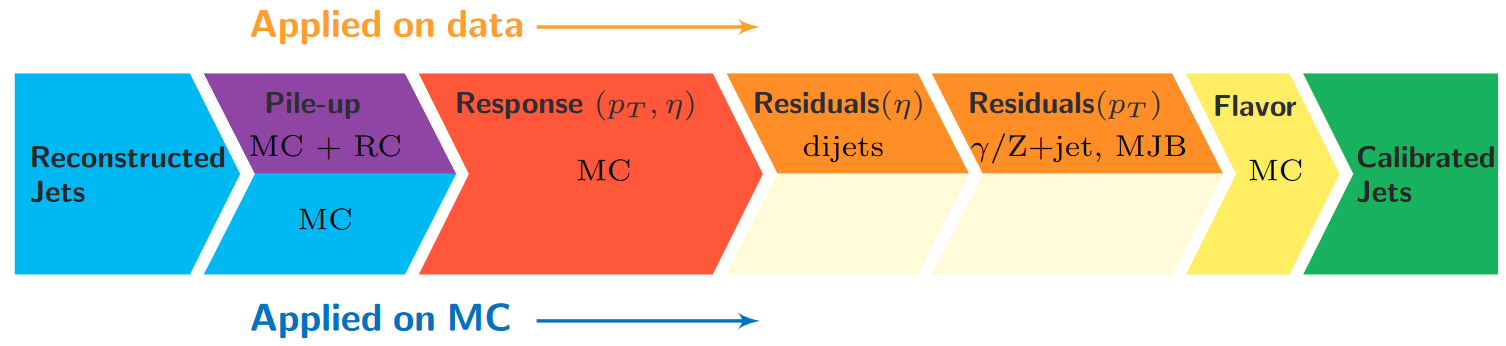
Particles from additional interactions in nearby bunch crossings of the LHC contribute energy in the calorimeters that must somehow be distinguished from the energy deposits of the main interaction. Extra energy in a jet’s cone can make its measured momentum larger than the momentum of the parent particle. The first layer (“L1”) of jet energy corrections accounts for pileup by subtracting the average transverse momentum contribution of the pileup interactions to the jet’s cone area. This average pileup contribution varies by pseudorapidity and, of course, by the number of interactions in the event.
The second and third layers of corrections (“L2L3”) correct the measured momentum to the true momentum as functions of momentum and pseudorapidity, bringing the reconstructed jet in line with the generated jet. These corrections are derived using momentum balancing and missing energy techniques in dijet and Z boson events. One well-measured object (ex: a jet near the center of the detector, a Z boson reconstructed from leptons) is balanced against a jet for which corrections are derived.
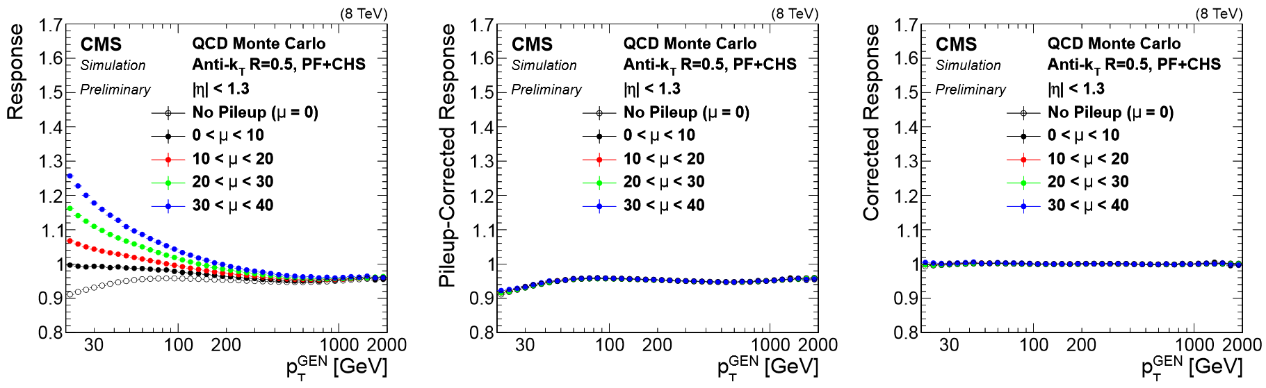
All of these corrections are applied to both data and simulation. Data events are then given “residual” corrections to bring data into line with the corrected simulation. A final set of flavor-based corrections are used in certain analyses that are especially sensitive to flavor effects. All of the corrections are described in this paper. The figure below shows the result of the L1+L2+L3 corrections on the jet response.
JEC from text files
There are several methods available for applying jet energy corrections to reconstructed jets. We have demonstrated a method to read in the corrections from text files and extract the corrections manually for each jet. The text files can be extracted from the global tag. First, set up sym links to the conditions databases for 2012 data and simulation (reference instructions):
Link database files
You might have done this in the pre-exercises! But if not, do it now. You will also need CVMFS mounted in your VM or docker container, which is covered in the pre-exercises.
$ ln -sf /cvmfs/cms-opendata-conddb.cern.ch/FT53_V21A_AN6_FULL FT53_V21A_AN6
$ ln -sf /cvmfs/cms-opendata-conddb.cern.ch/FT53_V21A_AN6_FULL.db FT53_V21A_AN6_FULL.db
$ ln -sf /cvmfs/cms-opendata-conddb.cern.ch/FT53_V21A_AN6_FULL FT53_V21A_AN6_FULL
$ ln -sf /cvmfs/cms-opendata-conddb.cern.ch/START53_V27 START53_V27
$ ln -sf /cvmfs/cms-opendata-conddb.cern.ch/START53_V27.db START53_V27.db
$ ls -l   ## make sure you see the full links as written above
To write out text files, we will use configs/jec_cfg.py, which uses a small analyzer to open the database files we just linked:
# connect to global tag
if isData:
    process.GlobalTag.connect = cms.string('sqlite_file:/cvmfs/cms-opendata-conddb.cern.ch/FT53_V21A_AN6_FULL.db')
    process.GlobalTag.globaltag = 'FT53_V21A_AN6::All'
else:
    process.GlobalTag.connect = cms.string('sqlite_file:/cvmfs/cms-opendata-conddb.cern.ch/START53_V27.db')
    process.GlobalTag.globaltag = 'START53_V27::All'


# setup JetCorrectorDBReader
process.maxEvents = cms.untracked.PSet(input=cms.untracked.int32(1))
process.source = cms.Source('EmptySource')
process.ak5 = cms.EDAnalyzer('JetCorrectorDBReader',
                             payloadName=cms.untracked.string('AK5PF'),
                             printScreen=cms.untracked.bool(False),
                             createTextFile=cms.untracked.bool(True))

if isData:
    process.ak5.globalTag = cms.untracked.string('FT53_V21A_AN6')
else:
    process.ak5.globalTag = cms.untracked.string('START53_V27')
Make the text files
Run this job once with
isData = Trueand once withisData = False(if you access the condition database for the first time, this will take a while). Then move the text files to thedata/directory:$ cmsRun configs/jec_cfg.py $ ## edit the file and flip isData $ cmsRun configs/jec_cfg.py $ mv *AK5PF.txt data/
In simulation_cfg.py the file names are passed to the AOD2NanoAOD analyzer:
process.aod2nanoaod = cms.EDAnalyzer("AOD2NanoAOD",
        jecL1Name = cms.FileInPath('workspace/AOD2NanoAODOutreachTool/data/START53_V27_L1FastJet_AK5PF.txt'),
        jecL2Name = cms.FileInPath('workspace/AOD2NanoAODOutreachTool/data/START53_V27_L2Relative_AK5PF.txt'),
        jecL3Name = cms.FileInPath('workspace/AOD2NanoAODOutreachTool/data/START53_V27_L3Absolute_AK5PF.txt'),
        jecUncName = cms.FileInPath('workspace/AOD2NanoAODOutreachTool/data/START53_V27_Uncertainty_AK5PF.txt'),
        isData = cms.bool(False)
In AOD2NanoAOD.cc the files are read to build a factorizedJetCorrector object from which the corrections can be accessed:
// Object definitions
bool isData;
std::vector<std::string> jecPayloadNames_;
std::string              jecL1_;
std::string              jecL2_;
std::string              jecL3_;
boost::shared_ptr<FactorizedJetCorrector> jec_;

// In the constructor the factorizedJetCorrected is set up
AOD2NanoAOD::AOD2NanoAOD(const edm::ParameterSet &iConfig){
  isData = iConfig.getParameter<bool>("isData");
  jecL1_ = iConfig.getParameter<edm::FileInPath>("jecL1Name").fullPath(); // JEC level payloads
  jecL2_ = iConfig.getParameter<edm::FileInPath>("jecL2Name").fullPath(); // JEC level payloads
  jecL3_ = iConfig.getParameter<edm::FileInPath>("jecL3Name").fullPath(); // JEC level payloads

  //Get the factorized jet corrector parameters.
  jecPayloadNames_.push_back(jecL1_);
  jecPayloadNames_.push_back(jecL2_);
  jecPayloadNames_.push_back(jecL3_);

  std::vector<JetCorrectorParameters> vPar;
  for ( std::vector<std::string>::const_iterator payloadBegin = jecPayloadNames_.begin(),
    payloadEnd = jecPayloadNames_.end(), ipayload = payloadBegin; ipayload != payloadEnd; ++ipayload ) {
    JetCorrectorParameters pars(*ipayload);
    vPar.push_back(pars);
    }

  // Make the FactorizedJetCorrector and Uncertainty
  jec_ = boost::shared_ptr<FactorizedJetCorrector> ( new FactorizedJetCorrector(vPar) );

  // ....function continues
}
In the analyze function the correction is evaluated for each jet. The correction depends on
the momentum, pseudorapidity, energy, and cone area of the jet, as well as the value of “rho” (the average momentum
per area) and number of interactions in the event. The correction is used to scale the momentum of the jet.
Handle<double> rhoHandle;
iEvent.getByLabel(InputTag("fixedGridRhoFastjetAll"), rhoHandle);

for (auto it = jets->begin(); it != jets->end(); it++) {
  if (it->pt() > jet_min_pt) {

    reco::Candidate::LorentzVector uncorrJet = it->p4();
    jec_->setJetEta( uncorrJet.eta() );
    jec_->setJetPt ( uncorrJet.pt() );
    jec_->setJetE  ( uncorrJet.energy() );
    jec_->setJetA  ( it->jetArea() );
    jec_->setRho   ( *(rhoHandle.product()) );
    jec_->setNPV   ( vertices->size() );

    double corr = jec_->getCorrection();

    value_jet_pt[value_jet_n] = it->pt();
    value_corr_jet_pt[value_jet_n] = corr * uncorrJet.pt();

  }
}
Challenge: add L2L3 residual corrections to data
In data, the L2L3 residual corrections should also be applied. Use the “isData” switch and set up
AOD2NanoAOD.ccanddata_cfg.pyto fully correct jets in data.Solution
When processing data, we need to open 4 text files rather than 3. This happens first in the config, which is actually missing ALL the text files right now! No switching is needed since we have a separate data config, but python if statements can be used if you want to have one configuration file for both data and simulation (left as an exercise to the reader). The text files for data start with “FT53” rather than “START53”:
process.aod2nanoaod = cms.EDAnalyzer("AOD2NanoAOD",
		      isData = cms.bool(True),
		      doPat = cms.bool(False),
		      jecL1Name = cms.FileInPath('workspace/AOD2NanoAODOutreachTool/data/FT53_V21A_AN6_L1FastJet_AK5PF.txt')
		      jecL2Name = cms.FileInPath('workspace/AOD2NanoAODOutreachTool/data/FT53_V21A_AN6_L2Relative_AK5PF.txt')
		      jecL3Name = cms.FileInPath('workspace/AOD2NanoAODOutreachTool/data/FT53_V21A_AN6_L3Absolute_AK5PF.txt')
		      jecResName = cms.FileInPath('workspace/AOD2NanoAODOutreachTool/data/FT53_V21A_AN6_L2L3Residual_AK5PF.txt')
		      jecUncName = cms.FileInPath('workspace/AOD2NanoAODOutreachTool/data/FT53_V21A_AN6_Uncertainty_AK5PF.txt')
		      )
In the source code we need to: teach the code about L2L3Residual, open that file only is
isData, and apply uncertainties only if!isData. The first task is done in the class definition:std::string jecL3_; std::string jecRes_;The second task is done in the constructor function of
AOD2NanoAOD:jecL3_ = iConfig.getParameter<edm::FileInPath>("jecL3Name").fullPath(); jecRes_ = iConfig.getParameter<edm::FileInPath>("jecResName").fullPath(); jecPayloadNames_.push_back(jecL3_); if(isData) jecPayloadNames_.push_back(jecRes_);And finally, we should escape the uncertainty calculation (more info on this below!) in the jet loop if we are working on data:
 double corrUp = 1.0;
 double corrDown = 1.0;
 if(!isData){
   jecUnc_->setJetEta( uncorrJet.eta() );
   // etc, through accessing corrUp and corrDown
 }
Jet Energy Resolution
These corrections account for differences between the true and measured energy scale of jets, but not the energy resolution. The jet momentum resolution is typically too small in simulation and is widened using a Gaussian smearing technique. Watch for implementation details on this correction in a future update to the Open Data Guide.
JEC while producing pat::Jets
Another popular object format in CMS is the “Physics Analysis Toolkit” format, called PAT. The jet energy corrections and Type-1 MET corrections can be
applied to RECO jets while making PAT jets. To do this we will load the global tag and databases directly in the configuration file and use the ‘addJetCollection’
process to create a collection of pat::jets. Look at simulation_patjets_cfg.py:
# Set up the new jet collection
process.ak5PFJets.doAreaFastjet = True
addPfMET(process, 'PF')

addJetCollection(process,cms.InputTag('ak5PFJets'),
                 'AK5', 'PFCorr',
                 doJTA        = True,
                 doBTagging   = True,
                 jetCorrLabel = ('AK5PF', cms.vstring(['L1FastJet','L2Relative','L3Absolute']))
                 doType1MET   = True,
                 doL1Cleaning = True,
                 doL1Counters = False,
                 doJetID      = True,
                 jetIdLabel   = "ak5",
                 )
In AOD2NanoAOD.cc we can look at the sections marked if(doPat) to see the difference in usage. In general, pat::jets are more
complex to create in the configuration file, but simpler to use because of their additional functions. In particular, accessing the
jet’s flavor directly makes calculation of b-tagging efficiencies and scale factors simpler.
  if(doPat){

    Handle<PFMETCollection> metT1;
    iEvent.getByLabel(InputTag("pfType1CorrectedMet"), metT1);
    value_met_type1_pt = metT1->begin()->pt();

    Handle<std::vector<pat::Jet> > patjets;
    iEvent.getByLabel(InputTag("selectedPatJetsAK5PFCorr"), patjets);

    value_patjet_n = 0;
    for (auto it = patjets->begin(); it != patjets->end(); it++) {
      if (it->pt() > jet_min_pt) {

        // Corrected values are now the default
        value_patjet_pt[value_patjet_n] = it->pt();
        value_patjet_eta[value_patjet_n] = it->eta();
        value_patjet_mass[value_patjet_n] = it->mass();

        // but uncorrected values can be accessed. JetID should be computed from the uncorrected jet
        pat::Jet uncorrJet = it->correctedJet(0);
        value_uncorr_patjet_pt[value_patjet_n] = uncorrJet.pt();
        value_uncorr_patjet_eta[value_patjet_n] = uncorrJet.eta();
        value_uncorr_patjet_mass[value_patjet_n] = uncorrJet.mass();

        // b-tagging is built in. Can access the truth flavor needed for b-tag effs & scale factor application!
        value_patjet_hflav[value_patjet_n] = it->hadronFlavour();
        value_patjet_btag[value_patjet_n] = it->bDiscriminator( "pfCombinedSecondaryVertexBJetTags");

        value_patjet_n++;
      }
    }
  }
Challenge: create PAT jets
Run
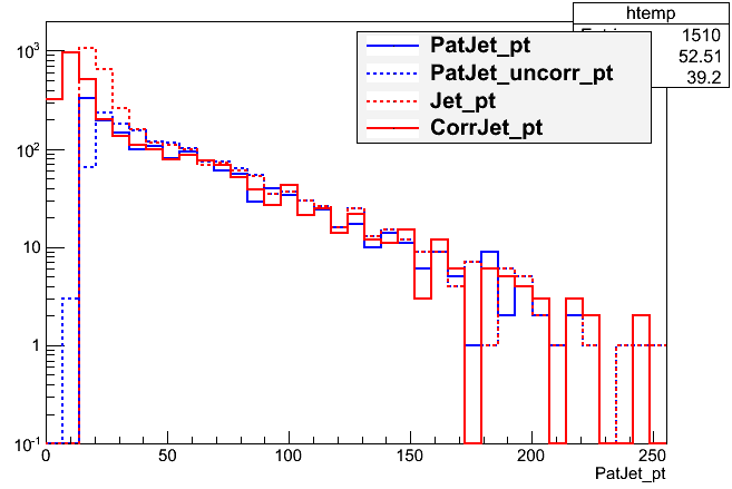
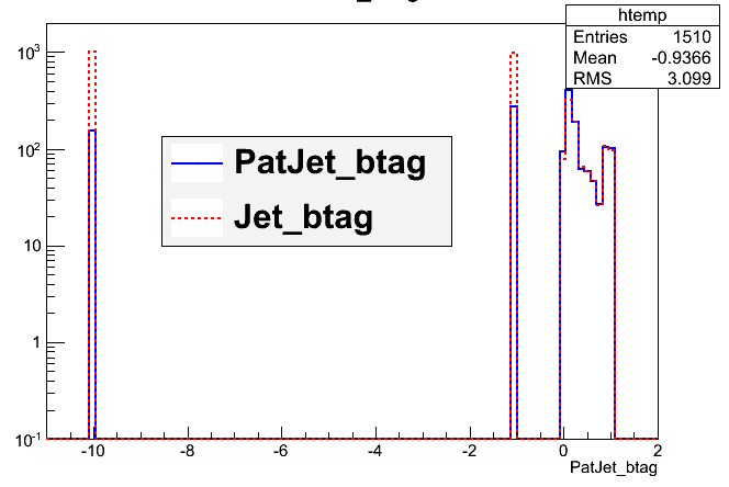
simulation_patjets_cfg.py, open the file, and compare the two jet correction and b-tagging methods. Method 1 hasJet_andCorrJet_branches and Method 2 hasPatJet_andPatJet_uncorrbranches.Solution
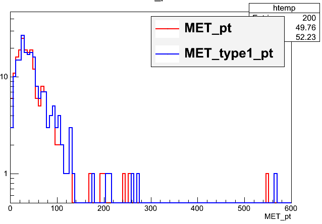
We can clearly see the difference between corrected and uncorrected jet momentum, particularly at low momentum where the effects of pileup are largest as a fraction of the total jet energy. here are differences in the number of jets across the collections because of different applications of the pt threshold (applied to uncorrected PFJets and corrected PATJets). We can also see small differences between particle-flow MET and type-1 corrected MET. The b-tagging distribution is almost identical, with the majority of the differences between the jet collections lying in the “dummy” value columns.
Uncertainties
You will have noticed that nested among the jet energy correction code snippets give above were commands related to the uncertainty in this correction. The uncertainty is also read from a text file in this example, and is used to increase or decrease the correction to the jet momentum.
// Object definition
boost::shared_ptr<FactorizedJetCorrector> jec_;

// In the constructor the JetCorrectionUncertainty is set up
AOD2NanoAOD::AOD2NanoAOD(const edm::ParameterSet &iConfig){

  jecUncName_ = iConfig.getParameter<edm::FileInPath>("jecUncName").fullPath();      // JEC uncertainties
  jecUnc_ = boost::shared_ptr<JetCorrectionUncertainty>( new JetCorrectionUncertainty(jecUncName_) );

  // ....function continues
}

// In the analyze function the uncertainty is evaluated
for (auto it = jets->begin(); it != jets->end(); it++) {
  if (it->pt() > jet_min_pt) {

    double corr = jec_->getCorrection();

    jecUnc_->setJetEta( uncorrJet.eta() );
    jecUnc_->setJetPt( corr * uncorrJet.pt() );
    double corrUp = corr * (1 + fabs(jecUnc_->getUncertainty(1)));
    double corrDown = corr * ( 1 - fabs(jecUnc_->getUncertainty(-1)) );

    value_corr_jet_ptUp[value_jet_n] = corrUp * uncorrJet.pt();
    value_corr_jet_ptDown[value_jet_n] = corrDown * uncorrJet.pt();

  }
}
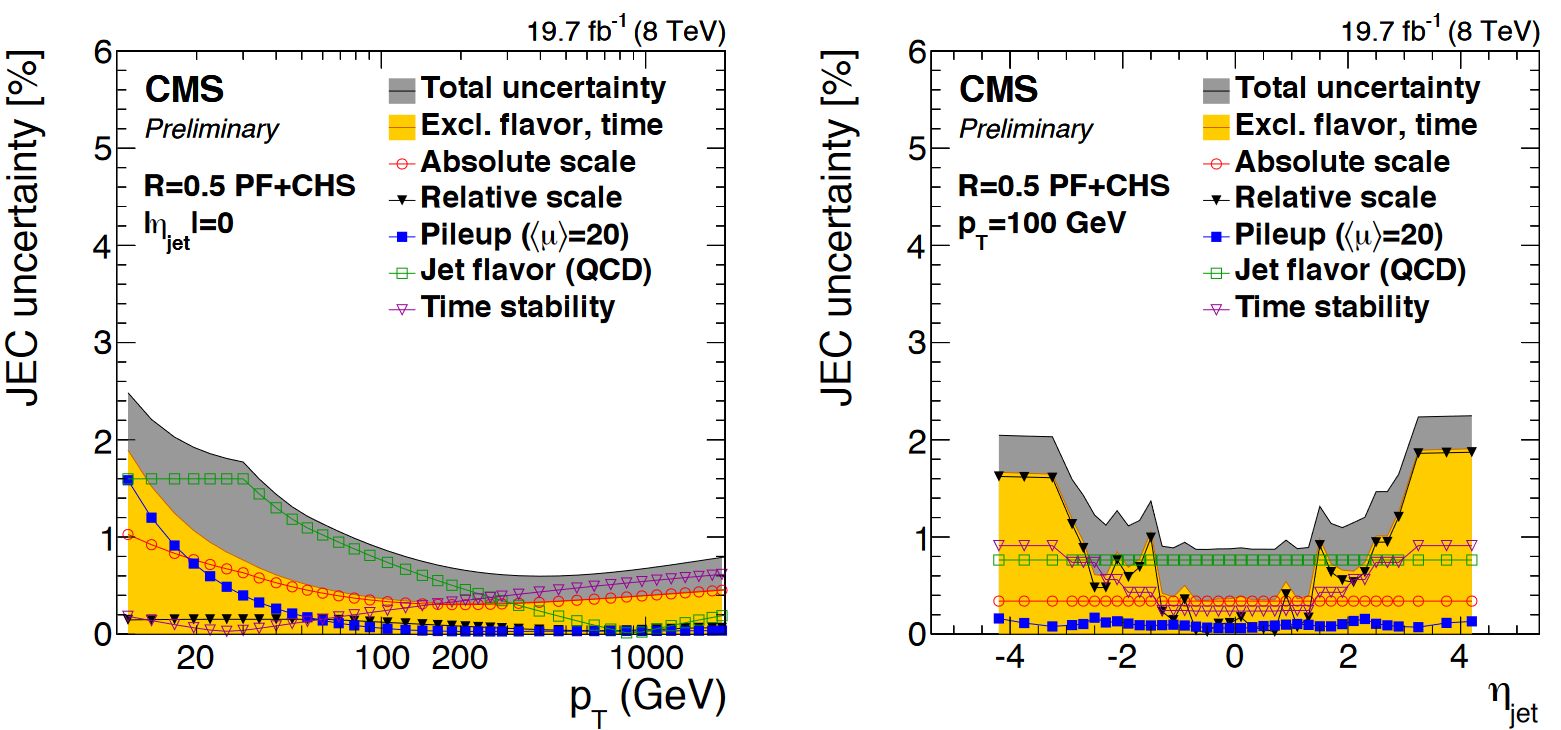
The uncertainties have several sources, shown in the figure below. The L1 (pileup) uncertainty dominates at low momentum, while the L3 (absolute scale) uncertainty takes over for higher momentum jets. All corrections are quite precise for jets located near the center of the CMS barrel region, and the precision drops as pseudorapidity increases and different subdetectors lose coverage.
Challenge: shifted histograms
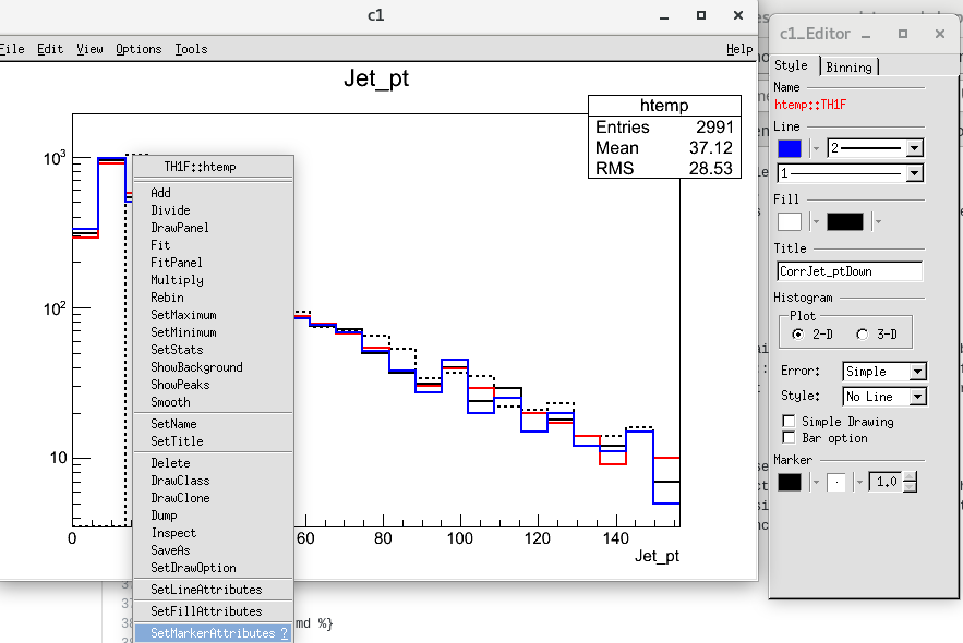
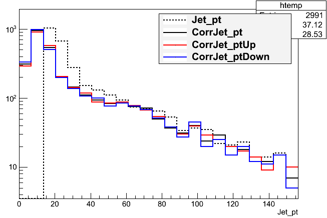
Plot and investigate the range of momentum variation given by the JEC uncertainties. Is the difference between the raw and corrected momentum larger or smaller than the uncertainty? Use TTree::Draw to make histograms of the various momentum distributions. Ideally, show the up and down variations in different colors, and the raw vs corrected momenta with different line styles.
Solution
Draw a histogram, hover over one of the lines, and right click. You should see a menu appear – select “Set Line Attributes” and a GUI with pop up. This is handy for changing line colors and styles interactively. Over the bulk of the momentum distribution, the jet energy corrections are significant – the corrected and uncorrected versions are not consistent within the uncertainty. Drawing these plots is a typical sanity check in CMS analyses to test whether the uncertainties look sensible.
Key Points
Jet energy corrections are factorized and account for many mismeasurement effects
L1+L2+L3 should be applied to jets used for analyses, with residual corrections for data
Jet energy corrections are an source of systematic error and uncertainties should be evaluated