Content from Introduction
Last updated on 2024-07-24 | Edit this page
Estimated time: 10 minutes
Overview
Questions
- Where do uncertainties come from in CMS analysis?
- How important are uncertainties to our results?
Objectives
- Identify the major types of uncertainties typically found in CMS analyses
- Review examples from papers of the impact of uncertainties on the physics results
All CMS algorithms are subject to uncertainty. Such is life!
Types of uncertainty
The typical CMS analysis will need to consider the following types of uncertainty:
- Statistical: uncertainty due to limited sample size, either in data or simulation.
-
Systematic: uncertainty due to any other source!
- Collisions: the luminosity collected by CMS carries an uncertainty of just over 1%, and the calculation of the number of simultaneous collisions per bunch crossing also has uncertainty.
- Theory: when using simulation, limited-order generation and the use of parton density functions contribute some uncertainty to the accuracy of the simulation.
- Detector: reconstruction algorithms used by CMS are never perfectly modeled by simulation. Correcting physics objects for imperfect detector response, applying identification algorithms, or even selecting events using trigger paths require calibration of how the decision affects data versus simulation. Computing adjustments to the simulation brings along uncertainties.
- Method: all analyses must choose how they will model background, calculate observables, etc. Many of these choices can contribute uncertainties.
The type of analysis determines which uncertainties are the most significant. Searches for new physics at high energies are often, but not always, limited by the available size of the dataset. This can make constraining systematic uncertainties less important than simply designing effective selection criteria to remove background events. Measurements of particle properties are often in the opposite regime – for many SM particles even partial CMS datasets already provide massive samples that are useful for precision measurements. The precision, and therefore the impact, of these measurements can depend heavily on making analysis choices that contribute the smallest possible uncertainties.
Top quark cross section measurement
The top quark cross section was measured in several different final states using the CMS 2016 dataset. The single lepton differential cross section measurement using this dataset shares a breakdown of all their uncertainties:
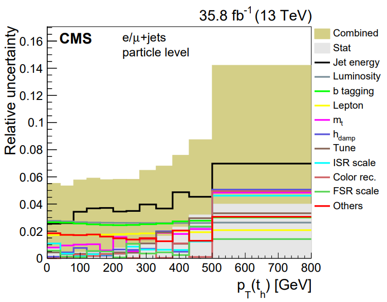
This figure shows that over a wide range of hadronic top quark momentum, the statistical uncertainty is completely negligible compared to systematic uncertainty. The experimental uncertainty groups (Jet energy, Luminosity, b tagging, and Lepton) tend to be larger than the other uncertainties, which are related to generation settings for the top pair simulation.
\(Z'\) search
The \(Z'\) search that we are using as an analysis inspiration uses many of the same individual uncertainties, but their impact is different. In this analysis the selection criteria are very stringent and few data events are left in the regions dominated by \(Z'\) signal:
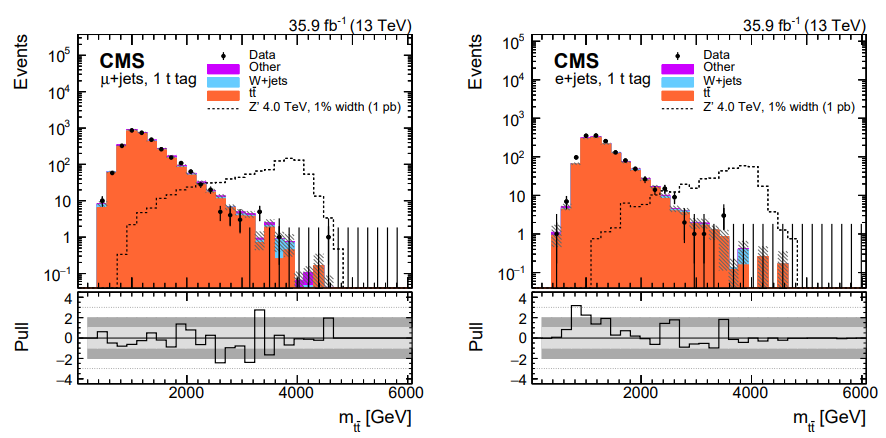
In fact, in order to perform the statistical inference for this analysis, these histograms had to be rebinned such that the statistical uncertainty stayed below 30% in each bin. The systematic uncertainties become less important in this search, especially for the higher mass signal. The authors note that including the systematic uncertainties in the fit at all have only a 10% effect on the mass limit for \(Z'\) masses above about 2 TeV.
In the following episodes we will look more closely at the different sources of CMS experimental uncertainty and practice evaluating some uncertainties in our analysis example.
Key Points
- Uncertainties are always divided into statistical and systematic components
- Many precision measurements also divide out luminosity and/or theory uncertainties
Content from Uncertainty sources
Last updated on 2024-07-31 | Edit this page
Estimated time: 30 minutes
Overview
Questions
- How are statistical uncertainties modeled in CMS for simulation and data?
- How are systematic uncertainties modeled in CMS?
- What are some of the most common uncertainties for CMS physics objects?
Objectives
- Learn what the error bars mean on CMS plots.
- Learn about collision, detector, and data-to-simulation correction uncertainties.
- Identify some published resources with more information.
Statistical uncertainties
Data: observations by CMS, such as the number of events in data that pass a certain set of selection criteria, are not in and of themselves uncertain. However, all CMS plots show error bars on data in histograms of observables. Let’s view again the image from the \(Z'\) search:
In this figure, many bins show an observation of 0 events in data, particularly in the high mass region. It is clear that this is not a fundamental statement that no events could ever be observed in those mass ranges, but merely a truth of this particular dataset collected by CMS in 2016.
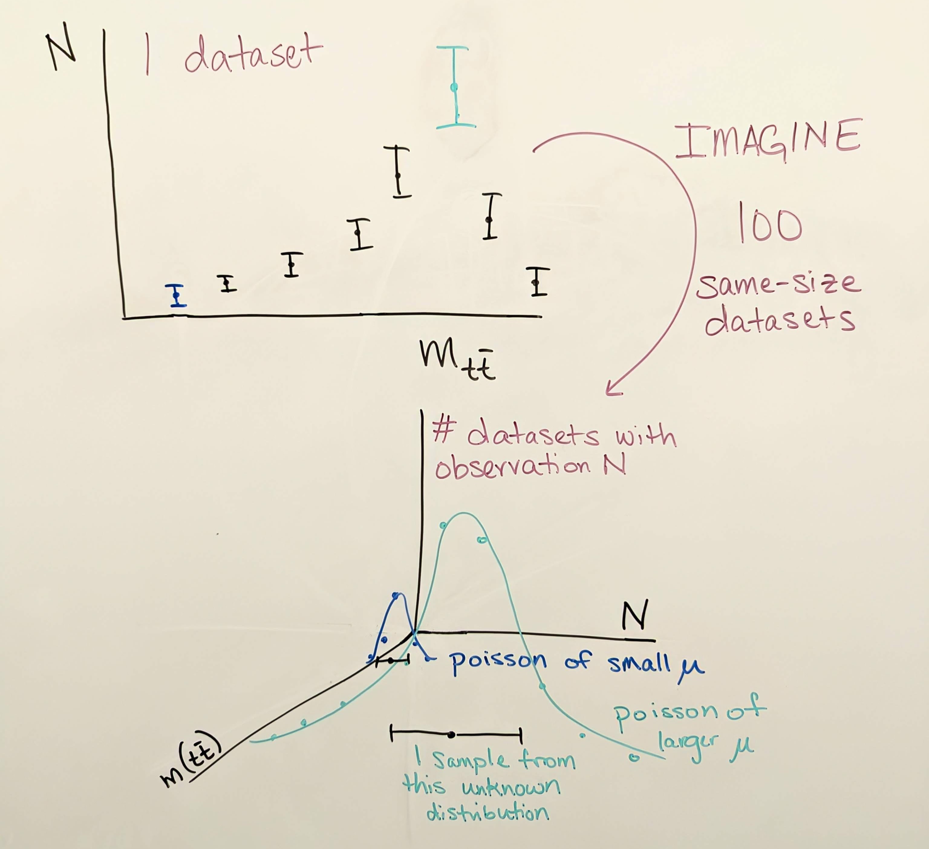
For any observable, such as the number of \(t\bar{t}\) events produced in CMS whose reconstructed mass lies in the 20th bin of the figure above, there is some “true” mean number of events per 35.9 fb\(^{-1}\) of data collected. This true mean number could perhaps be deduced by CMS repeating its 2016 data collection over and over again many times and finding in each dataset how many events lie in the 20th bin of this plot. But since we are analyzing just one iteration of 2016 data, we must let the observation in this dataset serve as our best estimate of the true mean. Each collision exhibiting a given set of properties is an independent random event, and so their probability follows the Poisson distribution, which has the unique feature that its standard deviation is the square root of the mean. If our best estimate of the true mean is the observation we have in hand, then our best estimate of the variance is the square root of the observation. This estimate is generally reasonable, until the observation becomes very small, such as zero events. In this case, the asymmetric shape of the Poisson distribution is better illustrated by an upward pointing error bar from 0 that describes a one-sided 68% confidence limit.
MC: similar to the argument for data, uncertainty due to the limited size of a simulated sample is typically the square root of the sum of squared weights in any given bin. The goal for simulation is to always have sufficient generated events for any sample that the weights are small.
Systematic uncertainties
While systematic uncertainties have many different sources and are computed in many differen ways, the general underlying assumption is that the variation of an observable due to systematic uncertainty can be described by the Gaussian distribution, or by a log-normal distribution if negative values are not physical. Experimental uncertainties are usually provided as “up” and “down” shifts of a parameter, with the assumption that the “up”/“down” settings model a variation of one standard deviation.
The following sections give a brief introduction to some of the most common experimental systematic uncertainties for CMS analyses. It is not an exhaustive list, but a good start.
Collision conditions
Luminosity: the luminosity uncertainty affects the number of predicted events for any simulated sample. A simulated sample is weighted based on (luminosity) \(\times\) (cross section) / (number of generated events), so uncertainty in the luminosity can be directly converted to uncertainty in the number of signal or background events in any observable. The luminosity uncertainty for 2016 data is 1.2%.
Pileup: in simulation, the number of simultaneous interactions per bunch crossing is modeled by Pythia, based on measurements of the total cross section for inelastic proton-proton scattering. In Pythia the typical inelastic cross section for 13 TeV collisions is 80 mb, while CMS measures 69.2 mb, with an uncertainty of 4.6%. Simulation is reweighted to the CMS inelastic cross section, and the uncertainty of 4.6% is propagated to analysis observables via a pair (“up” and “down”) of shifted weights.
Detector response corrections
Jet energy scale: The Physics Object pre-learning lesson describes the various individual corrections that make up the total “jet energy scale” correction. This set of corrections adjusts the calculation of jet energy and momentum to remove effects from pileup (extra energy in a jet) and imperfect detector response (too little energy in a jet). Each individual correction is a source of uncertainty – at minimum because the corrections are derived in limited-size samples.
The figure below shows JES uncertainties from Run 1. The L1 (pileup) correction uncertainty dominates at low momentum, while the L3 (absolute scale) correction uncertainty takes over for higher momentum jets. All corrections are quite precise for jets located near the center of the CMS barrel region, and the precision drops as pseudorapidity increases and different subdetectors lose coverage.
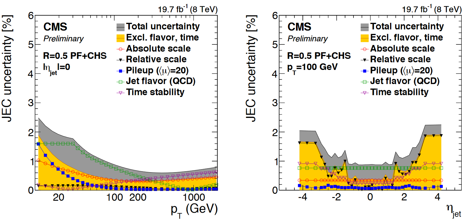
JES uncertainties modify the energy-momentum 4-vector of a jet, which tends to affect other overables in an analysis that are computed using jets or MET. These variations must be propagated all the way through to the final observable. CMS provides JES uncertainties as a total variation, and also from individual sources.
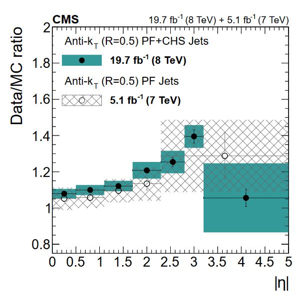
Jet energy resolution: The JER correction changes the width of the jet momentum distribution, rather than its position. The correction is provided as a set of “scale factors”, or multipliers, that affect the amount of Gaussian smearing applied to jet momentum in simulation. The scale factors in various pseudorapidity bins each have an uncertainty that comes from treatment of extra radiation in data, differences in MC generators, and other effects. The figure below shows the scale factors and their uncertainties from Run 1. Note how the larger data sample available for 8 TeV collisions corresponds to smaller uncertainties on the scale factors compared to 7 TeV! JER uncertainties also affect the energy-momentum 4-vector of a jet, independent from the JES variations!
Lepton energy scale and resolution: in precision measurements, leptons can also benefit from corrections for energy scale and resolution. While all analyses using jets must apply the JES corrections, not all analyses require these corrections for leptons. As the name suggests, CMS has a very strong muon detector and robust reconstruction algorithms, so extra muon energy corrections are not common. Similar for electrons – scale and smear studies are performed by the group responsible for electron reconstruction and identification, but they are not required for use in all analyses.
Lepton scale and resolution corrections affect the energy-momentum 4-vector of a lepton, so their uncertainties would be propagated to the final observable by repeating any calculations involving leptons using the energy/momentum variations. You can read more about the lepton energy scale measurements in the following papers:
- Muon performance: https://arxiv.org/abs/1804.04528
- Electron and photon performance: https://arxiv.org/abs/2012.06888
- Tau performance: https://arxiv.org/abs/1809.02816
Data/MC scale factors
What is a scale factor?
A “scale factor” is a number that should be multiplied onto some quantity so that it matches a different quantity. In CMS, scale factors usually adjust the event weight of a simulated event, so that histograms filled by simulated events match the histogram of the same observable in data.
Trigger: analysts often apply the same trigger path in data and simulation. But the efficiency of the trigger path depends on the kinematics of the physics objects used, and it might vary between data and simulation. Most analysts need to compute the efficiencies of the triggers they use, and then compute scale factors comparing data and simulation efficiencies. The uncertainty in each efficiency can be propagated to the scale factor, and then to the final analysis observable.
Leptons: selecting leptons usually involves choosing an identification criterion and an isolation criterion. The efficiency of these algorithms to identify “true” leptons can vary between simulation and data! For muons and electrons, scale factors are typically calculated using Z boson tag-and-probe, which was featured in an earlier workshop.
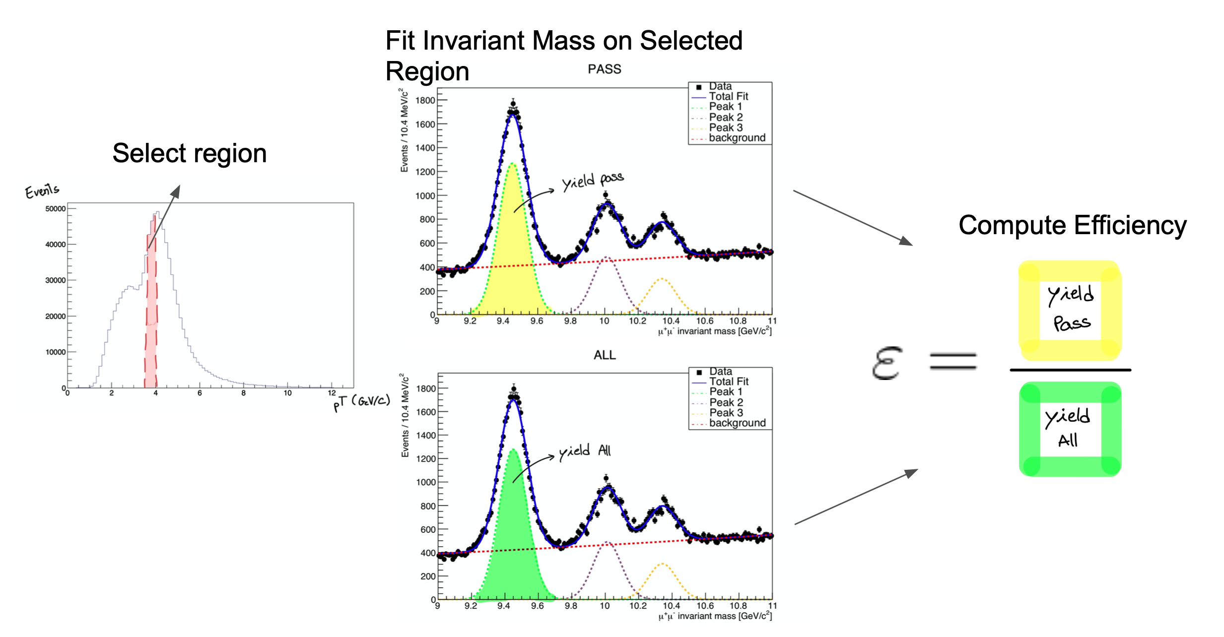
Tag and probe can be done with any 2-lepton resonance, such as \(J/\psi\) or \(\Upsilon\) mesons, though \(Z\) bosons are preferred for higher-momentum leptons. Events are selected with two leptons of the same flavor but opposite charge, and a stringent requirement is placed on the invariant mass of the lepton pair, so that we can be reasonably sure the event was “really” the desired resonance particle. For these events, we are then reasonably sure that both leptons are “true” signal leptons, not the result of detector noise. In the tag-and-probe process, the “tag” lepton is required to pass selection criteria that reject large fractions of “background” or “noise” leptons. The other lepton is the probe, and the rate at which it passes or fails any number of selection criteria can be tested. The figure below shows how distributions of the resonance mass are fitted to extract the number of particles whose probe lepton passed the criteria.
Uncertainties in scale factors calculated using the tag-and-probe procedure can come from a variety of sources:
- Change the binning of the histograms
- Change the resonance particle mass range accepted
- Change the functional form used to fit the signal
- Change the functional form used to fit the background
- Statistical uncertainty
- Uncertainty in the fit parameters
Thankfully, these variations usually result in only small changes to the efficiency and therefore the scale factor! They are usually combined in quadrature to one variation. You can read more in the lepton performance papers:
- Muon performance: https://arxiv.org/abs/1804.04528
- Electron and photon performance: https://arxiv.org/abs/2012.06888
- Tau performance: https://arxiv.org/abs/1809.02816
Jet identification: The jet identification algorithm designed to reject noise jets is usually 98-99% efficienct for true jets, and this efficiency tends to match between data and simulation, so most analyses do not include a scale factor or uncertainty for this algorithm. Yay!
However, jets more than make up for the efficiency of their noise-rejection ID with the complexity of the scale factors and uncertainties for parent-particle identification algoriths like b tagging, W tagging, or top tagging. The goal of scale factors for these algorithms is the same as all others: bring simulation to match data. But while “detector noise” versus “actual jet” is a fairly concrete question, “b quark jet” versus “c quark jet” is much more subtle. In simulation, where the “true” parent particles behind any jet can be determined, it is fairly straightforward to measure the efficiency with which true t, W, Higgs, Z, b, c, or light quark jets will pass a certain tagging criterion. But to measure the same in data, an event selection must be defined that can bring “reasonable certainty”, as we mentioned for tag-and-probe, that the jets considered are actually b quark jets, W boson jets, top quark jets, etc. As in the case of tag-and-probe, calculating these efficiencies will usually involve fits that bring in many sources of uncertainty. The uncertainties can vary based on jet kinematics and the jet’s parent particle.
Scale factors and their uncertainties for many jet identification algorithms in the 2016 dataset are documented in the following sources:
- Identification of b and c quarks: https://cds.cern.ch/record/2854609/
- Double-b identification for Higgs bosons: http://cds.cern.ch/record/2866276
- Heavy particle identification (H, W, t): https://arxiv.org/abs/2004.08262
Analysis method choices
Uncertainties for corrections to physics objects are often provided by CMS, at least for any required corrections, and for the most popular identification algorithms. But uncertainties also arise from analysis strategy choices. There is no way to write an exhaustive list of these uncertainties! But as you build an analysis, consider:
- Have I calculated any custom corrections for physics objects?
- Have I performed any fits to model background and/or signal?
- Have I computed any “transfer factors” to model background in a certain region using information from other regions?
- Have I designed a validation procedure for my background modeling strategy?
All of these methods, and surely others, will need to be evaluated for uncertainties that should be propagated to your final observable. Uncertainties in fit parameters, statistical uncertainties in various regions, any deviation from expectations in a validation procedure – all are examples of analysis method uncertainties you might find in CMS papers and consider in your work.
Key Points
- Data in CMS plots carry error bars that serve as a “best estimate” of the variance of the Poisson distribution that governs the expected observations for each observable.
- Systematic uncertainties are assumed to follow Gaussian or log-normal probability distributions.
- Collision-based uncertainties come from the luminosity and pileup calculations.
- Detector-based uncertainties come from corrections to the energy response for different physics objects.
- Scale factor-based uncertainties come from the calculation methods used to measure efficiencies for various reconstruction, identification, isolation, and trigger algorithms.
- Analysis methods also bring in uncertainties that need to be determined by the analysis team.
Content from Physics object corrections
Last updated on 2024-07-26 | Edit this page
Estimated time: 20 minutes
Overview
Questions
- What corrections are provided by CMS for pileup?
- What corrections are provided by CMS for leptons?
- What corrections are provided by CMS for jets and MET?
- How can I access the corrections?
Objectives
- Explore the corrections webpage for 2016 data.
- Install the framework used by CMS to apply the common experimental corrections.
- Learn how to access a correction and its numerical value.
2016 corrections webpage
Open this website in your browser! https://opendata.cern.ch/eos/opendata/cms/corrections/jsonpog-integration-summary/index.html
CMS provides all of the corrections that are “required” for sensible analysis results (in most cases), and also provides scale factors for some of the most common identification and isolation algorithms. Prior to 2016, these corrections were shared with analysts as histograms, via PDF files, via TWiki pages, or other forms, and each group calculating a correction could choose the format. For Run 2 data, a common JSON format has been introduced that simplifies and unifies the process of accessing correction values and their uncertainties.
Exploring the correction website
When you click on the website link above, you should see the following page:
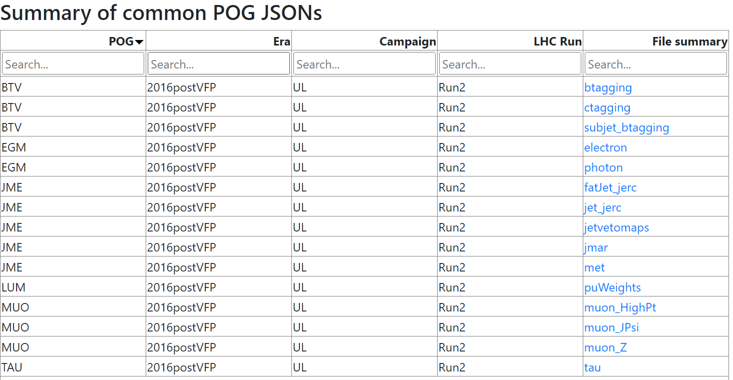
The columns describe:
- The acronym of the CMS group that produced the correction:
- BTV = B-tagging & vertexing
- EGM = E & Gamma (electrons & photons)
- JME = Jets & MET
- LUM = Luminosity, including pileup
- MUO = Muons
- TAU = Tau leptons
- Information about the CMS dataset:
- Era: currently, the page shows “2016postVFP”, which applies to the Run2016G and Run2016H data released in 2024. As we release more Run 2 data, additional eras will appear on this website.
- Campaign: “UL” = “Ultra-Legacy”. The open data released for 2016 is not the earliest processing of 2016 data, but the final processing that is uniform with the rest of the Run 2 data that will be released in coming years.
- LHC Run: Run 2! If you revisit this site in 2028 or 2029 you might begin to see some “Run 3” corrections.
- The files available with corrections. These are clickable links that take you to a summary page for the corrections contained within that file.
Correction file structure
Click on a correction file to explore it!
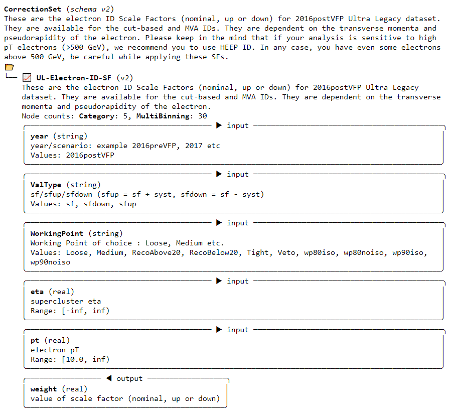
One of the simplest examples is the electron correction file. When clicking on that link, you see a description of the correction contained in the file:
Identify correction elements
Important information for accessing the correction in an analysis is included on this page. Look and find:
- The name of the correction
- The required input values: what information must you provide to get a correction value out of this JSON file? What types are the required inputs? What ranges can the inputs take?
- The expected output value: what piece of information will be returned by the correction? What type will it have?
For the electron correction, the name is “UL-Electron-ID-SF”. The “(v2)” that appears next to the name is indicating a version of the correction JSON software, and is not part of the name.
There are five input values required to access the electron correction:
- “year”: this is unfortunately a bit redundant, but you must provide the string “2016postVFP” when accessing this correction.
- “ValType”: this input allows you to specify whether you would like to access the scale factor (“sf”) or one of its systematic uncertainty variations (“sfdown”, “sfup”).
- “WorkingPoint”: this inputs allows you to specify which electron
identification algorithm you are using.
- “RecoAbove20”, “RecoBelow20”: these names will access scale factors for the electron reconstruction algorithm for electrons with energy either above or below 20 GeV.
- “Veto”, “Loose”, “Medium”, “Tight”: these are the working points of
the
Electron\_cutBasedidentification algorithm. - “wp80iso”, “wp80noiso”, “wp90iso”, “wp90noiso”: these are the
working points of the MVA identification algorithm. The number indicates
the efficiency for identifying true electrons (80% or 90%), and
“iso”/“noiso” indicates whether or not isolation was included in the
training variables for the MVA. In NanoAOD the branches for these
identification algorithms look like
Electron_mvaFall17V2*_WP*.
- The \(\eta\) and \(p_T\) values for the electron. Both are to
be provided as
floatvalues, and the electron’s \(p_T\) value must be larger than 10 GeV for the correction to be found.
The output will be a float that corresponds to a scale factor. The scale factor or one of its systematic variations should be multiplied onto the event weight. We will show this in an upcoming exercise.
Explore other correction files for jets, leptons, etc. The table below gives a basic map of what you expect to find in the different files:
| Correction type | Physics object | File |
|---|---|---|
| Collision | Pileup | puWeights |
| Detector response | Jets | jet_jerc, fatjet_jerc, jetvetomaps |
| Detector response | MET | met |
| Detector response | Taus | tau |
| Scale factors | Muons | muon_JPsi, muon_Z, muon_HighPt |
| Scale factors | Electrons | electron |
| Scale factors | Photons | photon |
| Scale factors | Taus | tau |
| Scale factors | Jets | btagging, ctagging, subjet_btagging, jmar |
Software for accessing corrections
Install correctionlib
Open your python docker container and install
correctionlib:
After pip installs any dependencies, you should see a
message that version 2.6.1 has been installed:
OUTPUT
Successfully installed correctionlib-2.6.1Download all the corrections files and unpack them:
BASH
wget https://opendata.cern.ch/eos/opendata/cms/corrections/jsonpog-integration-2016post.tar
tar -xf jsonpog-integration-2016post.tar
rm jsonpog-integration-2016post.tar
You should now see a folder called “POG” in your container with subdirectories for each CMS group:
OUTPUT
BTV EGM JME LUM MUO TAUIn the final episode, we will see how to use the
correctionlib package to access the corrections in the
files
Key Points
- The available 2016 corrections and a summary website can be accessed from the Open Data Portal (a “record” page for the corrections is forthcoming).
- Mandatory corrections such as pileup and jet energy corrections are provided.
- Scale factors for many reconstruction and identification algorithms are also provided.
- The summary webpage is the best reference to understand the names, inputs, and outputs of the corrections.
Content from Uncertainties challenge
Last updated on 2024-07-31 | Edit this page
Estimated time: 30 minutes
Overview
Questions
- How do I use correctionLib to evaluate a scale factor and its uncertainty?
- How do I propagate an uncertainty through my analysis?
Objectives
- Use correctionLib in the python environment to access scale factors.
- Compute shifted variables within the \(Z'\) analysis
- Store histograms in a ROOT file for the next lesson
The goal of this exercise is to use the correctionlib
tool to access some scale factors and apply them to our \(Z`\) search. We will also see one way to
store histograms in a ROOT file for use in the next lesson
on statistical inference.
Prerequisite
For the activities in this session you will need:
- Your python docker container and ROOT docker container
-
correctionlibinstalled in your python container - The
POG/folder of correction files - At least one
.csvfile produced in the lessons yesterday.
Just in case…
We think at this point everyone will have .csv files with our stored data. In case you don’t, download some example files into the shared folder of your Python container
BASH
wget https://github.com/cms-opendata-workshop/workshop2024-lesson-uncertainties/raw/main/instructors/SUMMED_Wjets.csv
wget https://github.com/cms-opendata-workshop/workshop2024-lesson-uncertainties/raw/main/instructors/SUMMED_collision.csv
wget https://github.com/cms-opendata-workshop/workshop2024-lesson-uncertainties/raw/main/instructors/SUMMED_signal_M2000.csv
wget https://raw.githubusercontent.com/cms-opendata-workshop/workshop2024-lesson-uncertainties/main/instructors/SUMMED_tthadronic.csv
wget https://github.com/cms-opendata-workshop/workshop2024-lesson-uncertainties/raw/main/instructors/SUMMED_ttleptonic.csv
wget https://github.com/cms-opendata-workshop/workshop2024-lesson-uncertainties/blob/main/instructors/SUMMED_ttsemilep.csv
wget https://github.com/cms-opendata-workshop/workshop2024-lesson-uncertainties/raw/main/instructors/output_signal_22BAB5D2-9E3F-E440-AB30-AE6DBFDF6C83.csv
Demo: muon scale factors
To show how to open and use a correction file, we will walk through the following notebook together as a demonstration. Download a notebook and launch jupyter-lab:
BASH
docker start -i my_python
code/$ wget https://raw.githubusercontent.com/cms-opendata-workshop/workshop2024-lesson-uncertainties/main/learners/CorrectionLib_demo.ipynb
code/$ jupyter-lab --ip=0.0.0.0 --no-browser
Double-click on this notebook in the file menu of jupyter-lab. This notebook shows how to access the scale factor for our muon identification algorithm.
Open a .csv file into an array
Replace the .csv file name below with one that you have in your container.
Get the input lists we need and evaluate the correction
The evaluate method in correctionlib is
used to access specific correction values. In python, this function uses
the syntax: evaluate(input 1, input 2, input 3, ...). The
inputs should be provided in the order they appear on the summary
webpage of the correction. The muon correction we are showing here
cannot accept numpy arrays inside the evaluate call, so we
will iterate over the input arrays.
Plot the effect of this uncertainty on the Z’ mass
PYTHON
plt.hist(muon_pt,bins=30,range=(0,600),weights=genWeight*leadmuon_sf,histtype="step",color="k",label="nominal")
plt.hist(muon_pt,bins=30,range=(0,600),weights=genWeight*leadmuon_sfup,histtype="step",color="r",label="up")
plt.hist(muon_pt,bins=30,range=(0,600),weights=genWeight*leadmuon_sfdn,histtype="step",color="b",label="down")
plt.legend()
plt.xlabel('muon pT (GeV)')
plt.ylabel('events / 20 GeV')
plt.show()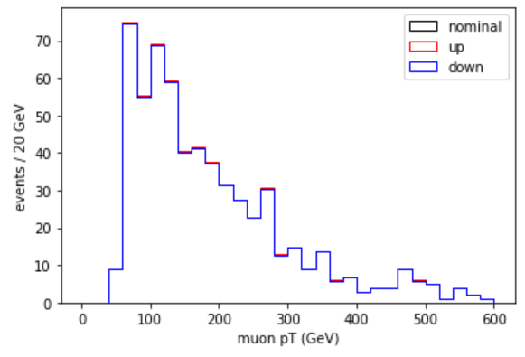
Exercise: implement pileup reweighting
Implement pileup reweighting
Follow the example of the previous notebook to implement pileup reweighting on your own!
Suggestions:
- Revisit the corrections website to learn the name of and inputs to the pileup correction
- Access any required inputs from your .csv file
- Adjust the muon example to read the correct file and access the right correction
You can work in the same notebook that you downloaded for the muon correction.
PYTHON
with gzip.open("POG/LUM/2016postVFP_UL/puWeights.json.gz",'rt') as file:
    data = file.read().strip()
    evaluator = correctionlib._core.CorrectionSet.from_string(data)

pileupcorr = evaluator["Collisions16_UltraLegacy_goldenJSON"]Plot the Z’ mass with the pileup weight applied, and its uncertainty shifts
PYTHON
plt.hist(signal['mtt'],bins=50,range=(0,3000),weights=genWeight*pu_sf,histtype="step",color="k",label="nominal")
plt.hist(signal['mtt'],bins=50,range=(0,3000),weights=genWeight*pu_sfup,histtype="step",color="r",label="up")
plt.hist(signal['mtt'],bins=50,range=(0,3000),weights=genWeight*pu_sfdn,histtype="step",color="b",label="down")
plt.legend()
plt.xlabel('m(tt) (GeV)')
plt.ylabel('events / 60 GeV')
plt.show()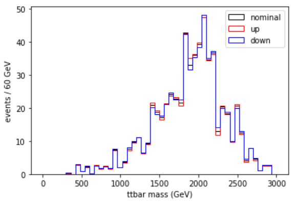
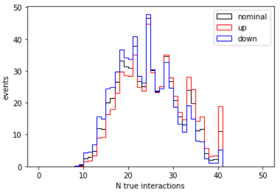
This uncertainty is larger than the muon scale factor uncertainty! It is also interesting to plot the uncertainty in the pileup distribution itself:
Demo: convert to ROOT histograms
To prepare for the final step of our analysis example, we need to
store our histograms in the ROOT file format. In
yesterday’s exercise to make a plot with data, background, and signal,
you saw some ways to handle information from multiple samples. This
example will be similar: we will read in the full .csv
output from the entire signal, background, and collision datasets and
produce a histogram. But this time we will also evaluate uncertainties
and convert the data to ROOT. Because our correctionlib
infrastructure lives in the python container, we will make histograms in
the python container, and then write them to a ROOT file in the ROOT
container.
Download the following notebook and follow along. In jupyter-lab, you can open a terminal to perform the download.
BASH
wget https://raw.githubusercontent.com/cms-opendata-workshop/workshop2024-lesson-uncertainties/main/learners/HistsWithWeights.ipynbWe will walk through this notebook together. It does not introduce any significant new skills or knowledge, but repeats the type of processing we have done before on multiple samples at once.
Read CSV files
First, we will open the .csv files we saved during the event selection process and store all the data in a dictionary. We will also create a dictionary to hold the number of events for each sample that we found in yesterday’s background modeling lesson. The keys of these dictionaries will be the types of data samples we are using in this search.
PYTHON
datadict = {}
datadict['signal'] = np.genfromtxt('SUMMED_signal_M2000.csv', delimiter=',', names=True, dtype=float)
datadict['tt_semilep'] = np.genfromtxt('SUMMED_ttsemilep.csv', delimiter=',', names=True, dtype=float)
datadict['tt_had'] = np.genfromtxt('SUMMED_tthadronic.csv', delimiter=',', names=True, dtype=float)
datadict['tt_lep'] = np.genfromtxt('SUMMED_ttleptonic.csv', delimiter=',', names=True, dtype=float)
datadict['wjets'] = np.genfromtxt('SUMMED_Wjets.csv', delimiter=',', names=True, dtype=float)
datadict['data'] = np.genfromtxt('SUMMED_collision.csv', delimiter=',', names=True, dtype=float)Open correctionlib files
Now we will load the two correctionlib JSON files that we used in the earlier examples, and access the specific corrections that we need.
PYTHON
import gzip
with gzip.open("POG/LUM/2016postVFP_UL/puWeights.json.gz",'rt') as file:
    data = file.read().strip()
    evaluator = correctionlib._core.CorrectionSet.from_string(data)
with gzip.open("POG/MUO/2016postVFP_UL/muon_Z.json.gz",'rt') as file:
    data = file.read().strip()
    evaluatorMU = correctionlib._core.CorrectionSet.from_string(data)

pucorr = evaluator["Collisions16_UltraLegacy_goldenJSON"]
mucorr = evaluatorMU["NUM_TightID_DEN_TrackerMuons"]
Store data for histograms
Now we will use the data we read from the .csv files to evaluate the 2 corrections and their uncertainties. We will slim down the number of variables that we need to create our final Z’ mass histograms and put everything in a final dictionary.
PYTHON
histoData = {}
for sample in datadict.keys():
    histoData[sample] = {
        "N_gen": N_gen[sample],
        "genWeight": datadict[sample]['weight']/np.abs(datadict[sample]['weight']),
        "mtt": datadict[sample]['mtt'],
        "pu_weight": [pucorr.evaluate(n,"nominal") for n in datadict[sample]['pileup']],
        "pu_weight_up": [pucorr.evaluate(n,"up") for n in datadict[sample]['pileup']],
        "pu_weight_dn": [pucorr.evaluate(n,"down") for n in datadict[sample]['pileup']],
        "muId_weight": [mucorr.evaluate(eta,pt,"nominal") for pt,eta in zip(datadict[sample]['mu_pt'],datadict[sample]['mu_abseta'])],
        "muId_weight_up": [mucorr.evaluate(eta,pt,"systup") for pt,eta in zip(datadict[sample]['mu_pt'],datadict[sample]['mu_abseta'])],
        "muId_weight_dn": [mucorr.evaluate(eta,pt,"systdown") for pt,eta in zip(datadict[sample]['mu_pt'],datadict[sample]['mu_abseta'])]
} Now we are ready to make our final histograms in ROOT. In your terminal (but not inside either docker container), copy your pickle file to the ROOT container’s shared folder, and then download the script that will save a ROOT file:
BASH
cp hists_for_ROOT.p ../cms_open_data_root/  ## Adjust if you have different paths
cd ../cms_open_data_root/
wget https://raw.githubusercontent.com/cms-opendata-workshop/workshop2024-lesson-uncertainties/main/learners/saveTH1F.py
Let’s investigate saveTH1F.py:
First, two modules are imported from ROOT:
Then we open the pickle file and extract the dictionary stored inside:
To store histograms with the correct relative weights, we will need their production cross sections, just as we saw in the plotting example.
PYTHON
xsec = {'signal':1.0,
        'tt_semilep':831.76*0.438,
        'tt_had':831.76*0.457,
        'tt_lep':831.76*0.105,
        'wjets':61526.7}
Now we can make ROOT’s TH1F objects and fill them with
our data. The TH1F object is constructed with 5 inputs: an
object name, a string containing the axis labels, the number of bins,
the lowest bin edge, and the highest bin edge.
Note a few things:
- Collision data is treated differently from the other samples. The
histogram’s name includes
data_obs. - Simulation is weighted by luminosity and cross section, but also by the individual event’s positive or negative weight and the correction factors that we extracted.
- Variation histograms for two uncertainty sources are stored. In these histograms one element of the event weight is adjusted.
PYTHON
roothists = {}
for sample in hists.keys():

    mtt = hists[sample]['mtt']

    if sample == "data":
        roothists[sample] = TH1F("mtt__data_obs",";m_{t#bar{t}} (GeV);events",50,0,3000)
        roothists[sample].FillN(len(mtt), mtt, np.ones(len(mtt)))
    else:
        genweight = hists[sample]['genWeight']
        Ngen = hists[sample]['N_gen']

        lumiweight = 16400*xsec[sample]*hists[sample]['genWeight']/Ngen
        weight = lumiweight*hists[sample]['pu_weight']*hists[sample]['muId_weight']
        pu_weight_up = lumiweight*hists[sample]['pu_weight_up']*hists[sample]['muId_weight']
        pu_weight_dn = lumiweight*hists[sample]['pu_weight_dn']*hists[sample]['muId_weight']
        muId_weight_up = lumiweight*hists[sample]['pu_weight']*hists[sample]['muId_weight_up']
        muId_weight_dn = lumiweight*hists[sample]['pu_weight']*hists[sample]['muId_weight_dn']

        roothists[sample+'_nominal'] = TH1F("mtt__"+sample,";m_{t#bar{t}} (GeV);events",50,0,3000)
        roothists[sample+'_nominal'].FillN(len(mtt), mtt, weight)
        roothists[sample+'_puUp'] = TH1F("mtt__"+sample+"__puUp",";m_{t#bar{t}} (GeV);events",50,0,3000)
        roothists[sample+'_puUp'].FillN(len(mtt), mtt, pu_weight_up)
        roothists[sample+'_puDn'] = TH1F("mtt__"+sample+"__puDown",";m_{t#bar{t}} (GeV);events",50,0,3000)
        roothists[sample+'_puDn'].FillN(len(mtt), mtt, pu_weight_dn)
        roothists[sample+'_muIdUp'] = TH1F("mtt__"+sample+"__muIdUp",";m_{t#bar{t}} (GeV);events",50,0,3000)
        roothists[sample+'_muIdUp'].FillN(len(mtt), mtt, muId_weight_up)
        roothists[sample+'_muIdDn'] = TH1F("mtt__"+sample+"__muIdDown",";m_{t#bar{t}} (GeV);events",50,0,3000)
        roothists[sample+'_muIdDn'].FillN(len(mtt), mtt, muId_weight_dn)
Finally, we will write all the TH1F objects in the
roothists dictionary to a ROOT file.
Enter your ROOT docker container and run the script:
When the script completes, you should be able to open the file in ROOT and list the contents:
The list should show all the histograms, including uncertainty shift histograms for simulation.
OUTPUT
TFile**         Zprime_hists_FULL.root
 TFile*         Zprime_hists_FULL.root
  KEY: TH1F     mtt__signal;1
  KEY: TH1F     mtt__signal__puUp;1
  KEY: TH1F     mtt__signal__puDown;1
  KEY: TH1F     mtt__signal__muIdUp;1
  KEY: TH1F     mtt__signal__muIdDown;1
  KEY: TH1F     mtt__tt_semilep;1
  KEY: TH1F     mtt__tt_semilep__puUp;1
  KEY: TH1F     mtt__tt_semilep__puDown;1
  KEY: TH1F     mtt__tt_semilep__muIdUp;1
  KEY: TH1F     mtt__tt_semilep__muIdDown;1
  KEY: TH1F     mtt__tt_had;1
  KEY: TH1F     mtt__tt_had__puUp;1
  KEY: TH1F     mtt__tt_had__puDown;1
  KEY: TH1F     mtt__tt_had__muIdUp;1
  KEY: TH1F     mtt__tt_had__muIdDown;1
  KEY: TH1F     mtt__tt_lep;1
  KEY: TH1F     mtt__tt_lep__puUp;1
  KEY: TH1F     mtt__tt_lep__puDown;1
  KEY: TH1F     mtt__tt_lep__muIdUp;1
  KEY: TH1F     mtt__tt_lep__muIdDown;1
  KEY: TH1F     mtt__wjets;1
  KEY: TH1F     mtt__wjets__puUp;1
  KEY: TH1F     mtt__wjets__puDown;1
  KEY: TH1F     mtt__wjets__muIdUp;1
  KEY: TH1F     mtt__wjets__muIdDown;1
  KEY: TH1F     mtt__data_obs;1
Exit ROOT with .q and you can exit the ROOT container.
In the final workshop lesson we will see how to use this type of ROOT
file to set a limit on the production cross section for the \(Z`\) boson.
What about all the other corrections and their uncertainties?
Examples of accessing and applying the other corrections found in the other JSON files will be included in the CMS Open Data Guide. Our goal is to complete this guide in 2024.
Key Points
- The correctionlib software provides a method to open and read corrections in the common JSON format.
- The
evaluatemethod takes in a correction’s required inputs and returns a correction value. - For event-weight corrections, save shifted event weight arrays to create shifted histograms.
- ROOT histograms can be created simply from arrays of data and weights for statistical analysis.