Uncertainties challenge
Last updated on 2024-07-31 | Edit this page
Estimated time: 30 minutes
Overview
Questions
- How do I use correctionLib to evaluate a scale factor and its uncertainty?
- How do I propagate an uncertainty through my analysis?
Objectives
- Use correctionLib in the python environment to access scale factors.
- Compute shifted variables within the \(Z'\) analysis
- Store histograms in a ROOT file for the next lesson
The goal of this exercise is to use the correctionlib
tool to access some scale factors and apply them to our \(Z`\) search. We will also see one way to
store histograms in a ROOT file for use in the next lesson
on statistical inference.
Prerequisite
For the activities in this session you will need:
- Your python docker container and ROOT docker container
-
correctionlibinstalled in your python container - The
POG/folder of correction files - At least one
.csvfile produced in the lessons yesterday.
Just in case…
We think at this point everyone will have .csv files with our stored data. In case you don’t, download some example files into the shared folder of your Python container
BASH
wget https://github.com/cms-opendata-workshop/workshop2024-lesson-uncertainties/raw/main/instructors/SUMMED_Wjets.csv
wget https://github.com/cms-opendata-workshop/workshop2024-lesson-uncertainties/raw/main/instructors/SUMMED_collision.csv
wget https://github.com/cms-opendata-workshop/workshop2024-lesson-uncertainties/raw/main/instructors/SUMMED_signal_M2000.csv
wget https://raw.githubusercontent.com/cms-opendata-workshop/workshop2024-lesson-uncertainties/main/instructors/SUMMED_tthadronic.csv
wget https://github.com/cms-opendata-workshop/workshop2024-lesson-uncertainties/raw/main/instructors/SUMMED_ttleptonic.csv
wget https://github.com/cms-opendata-workshop/workshop2024-lesson-uncertainties/blob/main/instructors/SUMMED_ttsemilep.csv
wget https://github.com/cms-opendata-workshop/workshop2024-lesson-uncertainties/raw/main/instructors/output_signal_22BAB5D2-9E3F-E440-AB30-AE6DBFDF6C83.csv
Demo: muon scale factors
To show how to open and use a correction file, we will walk through the following notebook together as a demonstration. Download a notebook and launch jupyter-lab:
BASH
docker start -i my_python
code/$ wget https://raw.githubusercontent.com/cms-opendata-workshop/workshop2024-lesson-uncertainties/main/learners/CorrectionLib_demo.ipynb
code/$ jupyter-lab --ip=0.0.0.0 --no-browser
Double-click on this notebook in the file menu of jupyter-lab. This notebook shows how to access the scale factor for our muon identification algorithm.
Open a .csv file into an array
Replace the .csv file name below with one that you have in your container.
Get the input lists we need and evaluate the correction
The evaluate method in correctionlib is
used to access specific correction values. In python, this function uses
the syntax: evaluate(input 1, input 2, input 3, ...). The
inputs should be provided in the order they appear on the summary
webpage of the correction. The muon correction we are showing here
cannot accept numpy arrays inside the evaluate call, so we
will iterate over the input arrays.
Plot the effect of this uncertainty on the Z’ mass
PYTHON
plt.hist(muon_pt,bins=30,range=(0,600),weights=genWeight*leadmuon_sf,histtype="step",color="k",label="nominal")
plt.hist(muon_pt,bins=30,range=(0,600),weights=genWeight*leadmuon_sfup,histtype="step",color="r",label="up")
plt.hist(muon_pt,bins=30,range=(0,600),weights=genWeight*leadmuon_sfdn,histtype="step",color="b",label="down")
plt.legend()
plt.xlabel('muon pT (GeV)')
plt.ylabel('events / 20 GeV')
plt.show()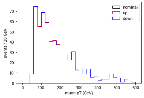
Exercise: implement pileup reweighting
Implement pileup reweighting
Follow the example of the previous notebook to implement pileup reweighting on your own!
Suggestions:
- Revisit the corrections website to learn the name of and inputs to the pileup correction
- Access any required inputs from your .csv file
- Adjust the muon example to read the correct file and access the right correction
You can work in the same notebook that you downloaded for the muon correction.
PYTHON
with gzip.open("POG/LUM/2016postVFP_UL/puWeights.json.gz",'rt') as file:
    data = file.read().strip()
    evaluator = correctionlib._core.CorrectionSet.from_string(data)

pileupcorr = evaluator["Collisions16_UltraLegacy_goldenJSON"]Plot the Z’ mass with the pileup weight applied, and its uncertainty shifts
PYTHON
plt.hist(signal['mtt'],bins=50,range=(0,3000),weights=genWeight*pu_sf,histtype="step",color="k",label="nominal")
plt.hist(signal['mtt'],bins=50,range=(0,3000),weights=genWeight*pu_sfup,histtype="step",color="r",label="up")
plt.hist(signal['mtt'],bins=50,range=(0,3000),weights=genWeight*pu_sfdn,histtype="step",color="b",label="down")
plt.legend()
plt.xlabel('m(tt) (GeV)')
plt.ylabel('events / 60 GeV')
plt.show()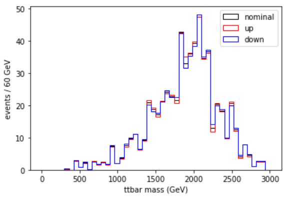
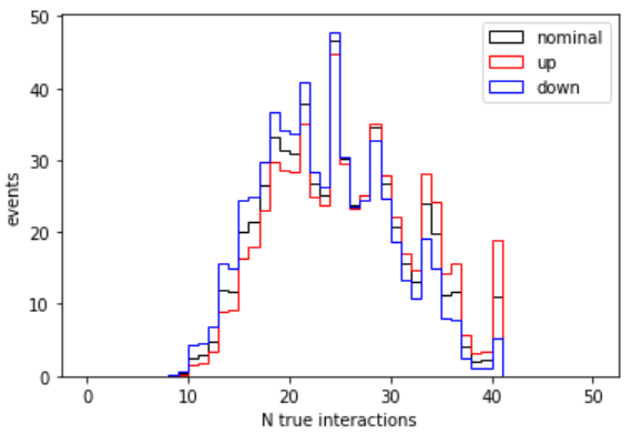
This uncertainty is larger than the muon scale factor uncertainty! It is also interesting to plot the uncertainty in the pileup distribution itself:
Demo: convert to ROOT histograms
To prepare for the final step of our analysis example, we need to
store our histograms in the ROOT file format. In
yesterday’s exercise to make a plot with data, background, and signal,
you saw some ways to handle information from multiple samples. This
example will be similar: we will read in the full .csv
output from the entire signal, background, and collision datasets and
produce a histogram. But this time we will also evaluate uncertainties
and convert the data to ROOT. Because our correctionlib
infrastructure lives in the python container, we will make histograms in
the python container, and then write them to a ROOT file in the ROOT
container.
Download the following notebook and follow along. In jupyter-lab, you can open a terminal to perform the download.
BASH
wget https://raw.githubusercontent.com/cms-opendata-workshop/workshop2024-lesson-uncertainties/main/learners/HistsWithWeights.ipynbWe will walk through this notebook together. It does not introduce any significant new skills or knowledge, but repeats the type of processing we have done before on multiple samples at once.
Read CSV files
First, we will open the .csv files we saved during the event selection process and store all the data in a dictionary. We will also create a dictionary to hold the number of events for each sample that we found in yesterday’s background modeling lesson. The keys of these dictionaries will be the types of data samples we are using in this search.
PYTHON
datadict = {}
datadict['signal'] = np.genfromtxt('SUMMED_signal_M2000.csv', delimiter=',', names=True, dtype=float)
datadict['tt_semilep'] = np.genfromtxt('SUMMED_ttsemilep.csv', delimiter=',', names=True, dtype=float)
datadict['tt_had'] = np.genfromtxt('SUMMED_tthadronic.csv', delimiter=',', names=True, dtype=float)
datadict['tt_lep'] = np.genfromtxt('SUMMED_ttleptonic.csv', delimiter=',', names=True, dtype=float)
datadict['wjets'] = np.genfromtxt('SUMMED_Wjets.csv', delimiter=',', names=True, dtype=float)
datadict['data'] = np.genfromtxt('SUMMED_collision.csv', delimiter=',', names=True, dtype=float)Open correctionlib files
Now we will load the two correctionlib JSON files that we used in the earlier examples, and access the specific corrections that we need.
PYTHON
import gzip
with gzip.open("POG/LUM/2016postVFP_UL/puWeights.json.gz",'rt') as file:
    data = file.read().strip()
    evaluator = correctionlib._core.CorrectionSet.from_string(data)
with gzip.open("POG/MUO/2016postVFP_UL/muon_Z.json.gz",'rt') as file:
    data = file.read().strip()
    evaluatorMU = correctionlib._core.CorrectionSet.from_string(data)

pucorr = evaluator["Collisions16_UltraLegacy_goldenJSON"]
mucorr = evaluatorMU["NUM_TightID_DEN_TrackerMuons"]
Store data for histograms
Now we will use the data we read from the .csv files to evaluate the 2 corrections and their uncertainties. We will slim down the number of variables that we need to create our final Z’ mass histograms and put everything in a final dictionary.
PYTHON
histoData = {}
for sample in datadict.keys():
    histoData[sample] = {
        "N_gen": N_gen[sample],
        "genWeight": datadict[sample]['weight']/np.abs(datadict[sample]['weight']),
        "mtt": datadict[sample]['mtt'],
        "pu_weight": [pucorr.evaluate(n,"nominal") for n in datadict[sample]['pileup']],
        "pu_weight_up": [pucorr.evaluate(n,"up") for n in datadict[sample]['pileup']],
        "pu_weight_dn": [pucorr.evaluate(n,"down") for n in datadict[sample]['pileup']],
        "muId_weight": [mucorr.evaluate(eta,pt,"nominal") for pt,eta in zip(datadict[sample]['mu_pt'],datadict[sample]['mu_abseta'])],
        "muId_weight_up": [mucorr.evaluate(eta,pt,"systup") for pt,eta in zip(datadict[sample]['mu_pt'],datadict[sample]['mu_abseta'])],
        "muId_weight_dn": [mucorr.evaluate(eta,pt,"systdown") for pt,eta in zip(datadict[sample]['mu_pt'],datadict[sample]['mu_abseta'])]
} Now we are ready to make our final histograms in ROOT. In your terminal (but not inside either docker container), copy your pickle file to the ROOT container’s shared folder, and then download the script that will save a ROOT file:
BASH
cp hists_for_ROOT.p ../cms_open_data_root/  ## Adjust if you have different paths
cd ../cms_open_data_root/
wget https://raw.githubusercontent.com/cms-opendata-workshop/workshop2024-lesson-uncertainties/main/learners/saveTH1F.py
Let’s investigate saveTH1F.py:
First, two modules are imported from ROOT:
Then we open the pickle file and extract the dictionary stored inside:
To store histograms with the correct relative weights, we will need their production cross sections, just as we saw in the plotting example.
PYTHON
xsec = {'signal':1.0,
        'tt_semilep':831.76*0.438,
        'tt_had':831.76*0.457,
        'tt_lep':831.76*0.105,
        'wjets':61526.7}
Now we can make ROOT’s TH1F objects and fill them with
our data. The TH1F object is constructed with 5 inputs: an
object name, a string containing the axis labels, the number of bins,
the lowest bin edge, and the highest bin edge.
Note a few things:
- Collision data is treated differently from the other samples. The
histogram’s name includes
data_obs. - Simulation is weighted by luminosity and cross section, but also by the individual event’s positive or negative weight and the correction factors that we extracted.
- Variation histograms for two uncertainty sources are stored. In these histograms one element of the event weight is adjusted.
PYTHON
roothists = {}
for sample in hists.keys():

    mtt = hists[sample]['mtt']

    if sample == "data":
        roothists[sample] = TH1F("mtt__data_obs",";m_{t#bar{t}} (GeV);events",50,0,3000)
        roothists[sample].FillN(len(mtt), mtt, np.ones(len(mtt)))
    else:
        genweight = hists[sample]['genWeight']
        Ngen = hists[sample]['N_gen']

        lumiweight = 16400*xsec[sample]*hists[sample]['genWeight']/Ngen
        weight = lumiweight*hists[sample]['pu_weight']*hists[sample]['muId_weight']
        pu_weight_up = lumiweight*hists[sample]['pu_weight_up']*hists[sample]['muId_weight']
        pu_weight_dn = lumiweight*hists[sample]['pu_weight_dn']*hists[sample]['muId_weight']
        muId_weight_up = lumiweight*hists[sample]['pu_weight']*hists[sample]['muId_weight_up']
        muId_weight_dn = lumiweight*hists[sample]['pu_weight']*hists[sample]['muId_weight_dn']

        roothists[sample+'_nominal'] = TH1F("mtt__"+sample,";m_{t#bar{t}} (GeV);events",50,0,3000)
        roothists[sample+'_nominal'].FillN(len(mtt), mtt, weight)
        roothists[sample+'_puUp'] = TH1F("mtt__"+sample+"__puUp",";m_{t#bar{t}} (GeV);events",50,0,3000)
        roothists[sample+'_puUp'].FillN(len(mtt), mtt, pu_weight_up)
        roothists[sample+'_puDn'] = TH1F("mtt__"+sample+"__puDown",";m_{t#bar{t}} (GeV);events",50,0,3000)
        roothists[sample+'_puDn'].FillN(len(mtt), mtt, pu_weight_dn)
        roothists[sample+'_muIdUp'] = TH1F("mtt__"+sample+"__muIdUp",";m_{t#bar{t}} (GeV);events",50,0,3000)
        roothists[sample+'_muIdUp'].FillN(len(mtt), mtt, muId_weight_up)
        roothists[sample+'_muIdDn'] = TH1F("mtt__"+sample+"__muIdDown",";m_{t#bar{t}} (GeV);events",50,0,3000)
        roothists[sample+'_muIdDn'].FillN(len(mtt), mtt, muId_weight_dn)
Finally, we will write all the TH1F objects in the
roothists dictionary to a ROOT file.
Enter your ROOT docker container and run the script:
When the script completes, you should be able to open the file in ROOT and list the contents:
The list should show all the histograms, including uncertainty shift histograms for simulation.
OUTPUT
TFile**         Zprime_hists_FULL.root
 TFile*         Zprime_hists_FULL.root
  KEY: TH1F     mtt__signal;1
  KEY: TH1F     mtt__signal__puUp;1
  KEY: TH1F     mtt__signal__puDown;1
  KEY: TH1F     mtt__signal__muIdUp;1
  KEY: TH1F     mtt__signal__muIdDown;1
  KEY: TH1F     mtt__tt_semilep;1
  KEY: TH1F     mtt__tt_semilep__puUp;1
  KEY: TH1F     mtt__tt_semilep__puDown;1
  KEY: TH1F     mtt__tt_semilep__muIdUp;1
  KEY: TH1F     mtt__tt_semilep__muIdDown;1
  KEY: TH1F     mtt__tt_had;1
  KEY: TH1F     mtt__tt_had__puUp;1
  KEY: TH1F     mtt__tt_had__puDown;1
  KEY: TH1F     mtt__tt_had__muIdUp;1
  KEY: TH1F     mtt__tt_had__muIdDown;1
  KEY: TH1F     mtt__tt_lep;1
  KEY: TH1F     mtt__tt_lep__puUp;1
  KEY: TH1F     mtt__tt_lep__puDown;1
  KEY: TH1F     mtt__tt_lep__muIdUp;1
  KEY: TH1F     mtt__tt_lep__muIdDown;1
  KEY: TH1F     mtt__wjets;1
  KEY: TH1F     mtt__wjets__puUp;1
  KEY: TH1F     mtt__wjets__puDown;1
  KEY: TH1F     mtt__wjets__muIdUp;1
  KEY: TH1F     mtt__wjets__muIdDown;1
  KEY: TH1F     mtt__data_obs;1
Exit ROOT with .q and you can exit the ROOT container.
In the final workshop lesson we will see how to use this type of ROOT
file to set a limit on the production cross section for the \(Z`\) boson.
What about all the other corrections and their uncertainties?
Examples of accessing and applying the other corrections found in the other JSON files will be included in the CMS Open Data Guide. Our goal is to complete this guide in 2024.
Key Points
- The correctionlib software provides a method to open and read corrections in the common JSON format.
- The
evaluatemethod takes in a correction’s required inputs and returns a correction value. - For event-weight corrections, save shifted event weight arrays to create shifted histograms.
- ROOT histograms can be created simply from arrays of data and weights for statistical analysis.