Introduction

Overview

Teaching: 10 min
Exercises: 0 min

Questions

How do we calculate efficiencies for the identification of physics objects?

What is the tag and probe method for calculating efficiencies?

Objectives

Understand the kind of efficiency measurements we are pursuing in this tutorial.

Learn what the tag and probe method is.

What is the tag and probe method?

The tag and probe method is a data-driven technique for measuring particle detection efficiencies. It is based on the decays of known resonances (e.g. J/ψ, ϒ and Z) to pairs of the particles being studied. In this exercise, these particles are muons, and the ϒ(1S) resonance is nominally used.

The determination of the detector efficiency is a critical ingredient in any physics measurement. It accounts for the particles that were produced in the collision but escaped detection (did not reach the detector elements, were missed by the reconstructions algorithms, etc). It can be in general estimated using simulations, but simulations need to be calibrated with data. The T&P method here described provides a useful and elegant mechanism for extracting efficiencies directly from data!.

What is “tag” and “probe”?

The resonance, used to calculate the efficiencies, decays to a pair of particles: the tag and the probe.

Tag muon = well identified, triggered muon (tight selection criteria).
Probe muon = unbiased set of muon candidates (very loose selection criteria), either passing or failing the criteria for which the efficiency is to be measured.

How do we calculate the efficiency?

The efficiency is given by the fraction of probe muons that pass a given criteria (in this case, the Muon ID which we explain below):

Efficiency equation

The denominator corresponds to the number of resonance candidates (tag+probe pairs) reconstructed in the dataset. The numerator corresponds to the subset for which the probe passes the criteria.

The tag+probe invariant mass distribution is used to select only signal, that is, only true Y(1S) candidates decaying to dimuons. This is achieved in this exercise by the usage of two methods: fitting and side-band-subtraction.

CMS Muon identification and reconstruction

The final objective in this lesson is to measure the efficiency for identifying reconstructed tracker muons. We present here a short description of the muon identification and reconstruction employed in the CMS experiment at the LHC.

CMS muon id

In the standard CMS reconstruction for proton-proton collisions, tracks are first reconstructed independently in the inner tracker and in the muon system. Based on these objects, two reconstruction approaches are used:

Tracker Muon reconstruction (red line): In this approach, all tracker tracks with pT > 0.5 GeV/c and total momentum p > 2.5 GeV/c are considered as possible muon candidates and are extrapolated to the muon system taking into account the magnetic field;
Standalone Muon reconstruction (green line): they are all tracks of the segments reconstructed in the muon chambers (performed using segments and hits from Drift Tubes - DTs in the barrel region, Cathode strip chambers - CSCs in the endcaps and Resistive Plates Chambers - RPCs for all muon system) are used to generate “seeds” consisting of position and direction vectors and an estimate of the muon transverse momentum;
Global Muon reconstruction (blue line): For each standalone-muon track, a matching tracker track is found by comparing parameters of the two tracks propagated onto a common surface.

You can find more details concerning CMS Muon Identification and reconstruction in this paper JINST 7 (2012) P10002.

Key Points

The efficiency we are pursuing in this lesson is for tracker muons.

Tag and probe are labels for each muon from a dimuon resonance, which are used for the calculation of efficiencies.

Tag is a biased particle while probe are unbiased.

The Fitting Method

Overview

Teaching: 20 min
Exercises: 10 min

Questions

What is the fitting method?

How do we use it to calculate the efficiency we are interested in (identification of tracker muons)?

Objectives

Understand the fitting method, it’s advantages and disadvantages

Learn how to implement this method using ROOT libraries in C++

Setting it up

In order to run this exercise you do not really need to be in a CMSSW area. It would be actually better if you worked outside your usual CMSSW_5_3_32 environment. So, if, for instance, you are working with the Docker container, instead of working on /home/cmsusr/CMSSW_5_3_32/src you could work on any directory you can create at the /home/cmsusr level. Alternatively, you could work directly on your own host machine if you managed to install ROOT on it.

For this example we assume you will be working in either the Docker container or the virtual machine.

Since we will be needing ROOT version greater than 6, then do not forget to set it up from LCG (as you learned in the ROOT pre-exercise) by doing:

source /cvmfs/sft.cern.ch/lcg/views/LCG_95/x86_64-slc6-gcc8-opt/setup.sh

Clone the repository and go to the tutorial:

git clone git://github.com/AthomsG/CMS-tutorial
cd CMS-tutorial/

A brief explanation of this repository

In this repository, you are only required to make changes to the Efficiency.C macro. These changes are highlighted as such:

/*-----------------------------------I N S E R T    C O D E    H E R E-----------------------------------*/

So when you see this comment, know that it’s your turn to code! If you don’t, the macro won’t run and the following errors are to be expected:

In file included from input_line_11:1:
/Users/thomasgaehtgens/Desktop/CMS-tutorial/Efficiency.C:13:23: error: expected expression
    bool DataIsMC   = ... ;
                      ^
/Users/thomasgaehtgens/Desktop/CMS-tutorial/Efficiency.C:15:23: error: expected expression
    string MuonId   = ... ;
                      ^
/Users/thomasgaehtgens/Desktop/CMS-tutorial/Efficiency.C:17:23: error: expected expression
    string quantity = ... ; //Pt, Eta or Phi
                      ^
/Users/thomasgaehtgens/Desktop/CMS-tutorial/Efficiency.C:25:22: error: expected expression
    double bins[] = {...};
                     ^
/Users/thomasgaehtgens/Desktop/CMS-tutorial/Efficiency.C:26:21: error: expected expression
    int bin_n     = ...;
                    ^
/Users/thomasgaehtgens/Desktop/CMS-tutorial/Efficiency.C:33:35: error: expected expression
    init_conditions[0] = /*peak1*/;
                                  ^
/Users/thomasgaehtgens/Desktop/CMS-tutorial/Efficiency.C:34:35: error: expected expression
    init_conditions[1] = /*peak2*/;
                                  ^
/Users/thomasgaehtgens/Desktop/CMS-tutorial/Efficiency.C:35:35: error: expected expression
    init_conditions[2] = /*peak3*/;
                                  ^
/Users/thomasgaehtgens/Desktop/CMS-tutorial/Efficiency.C:36:35: error: expected expression
    init_conditions[3] = /*sigma*/;

The Fitting Method

First, a brief explanation of the method we’ll be studying.

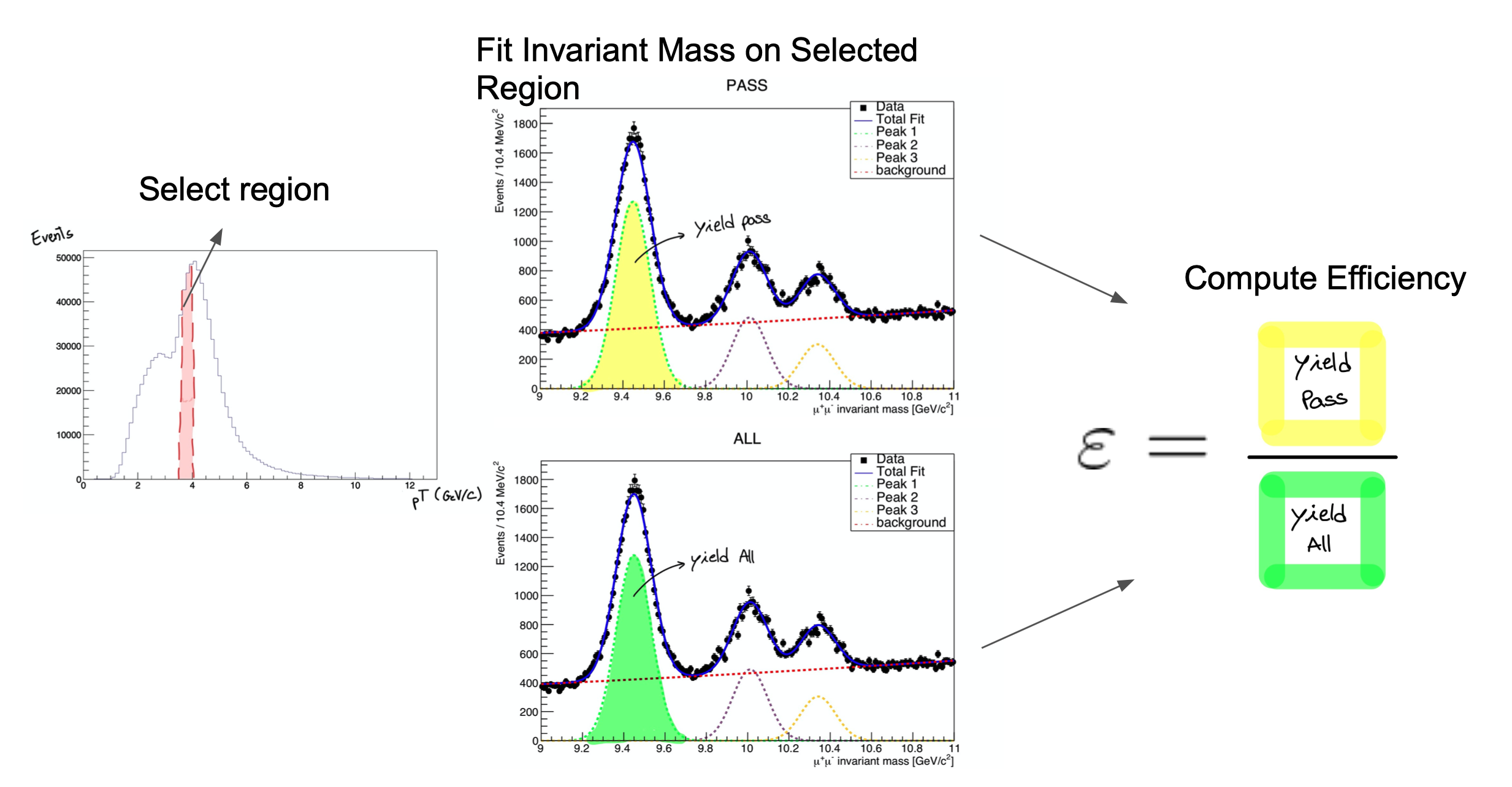
It consists on fitting the invariant mass of the tag & probe pairs, in the two categories: passing probes, and all probes. I.e., for the unbiased leg of the decay, one can apply a selection criteria (a set of cuts) and determine whether the object passes those criteria or not.

The procedure is applied after splitting the data in bins of a kinematic variable of the probe object (e.g. the traverse momentum, p_T); as such, the efficiency will be measured as a function of that quantity for each of the bins.

So, in the picture below, on the left, let’s imagine that the p_T bin we are selecting is the one marked in red. But, of course, in that bin (like in the rest) you will have true ϒ decays as well as muon pairs from other processes (maybe QCD, for instance). The true decays would make up our signal, whereas the other events will be considered the background.

The fit, which is made in a different space (the invariant mass space) allows to statistically discriminate between signal and background. To compute the efficiency we simply divide the signal yield from the fits to the passing category by the signal yield from the fit of the inclusive (All) category. This approach is depicted in the middle and right-hand plots of the image below.

At the end of the day, then, you will have to make these fits for each bin in the range of interest.

Let’s start exploring our dataset. From the cloned directory, type:

cd DATA/Upsilon/trackerMuon/
root -l T\&P_UPSILON_DATA.root

If everything’s right, you should get something like:

Attaching file T&P_UPSILON_DATA.root as _file0...
U(TFile *) 0x7fe2f34ca270

Of course, you can explore this file, if you want, using all the tools you learn in the ROOT pre-exercise. This file contains ntuples that were obtained using procedures similar to the ones you have been learning in this workshop.

In the following plots, remember that the units of the x axis are in GeV/c.

Now, before we start fitting the invariant mass it’s important to look at it’s shape first. To visualize our data’s invariant mass, do (within ROOT):

root [] UPSILON_DATA->Draw("InvariantMass")

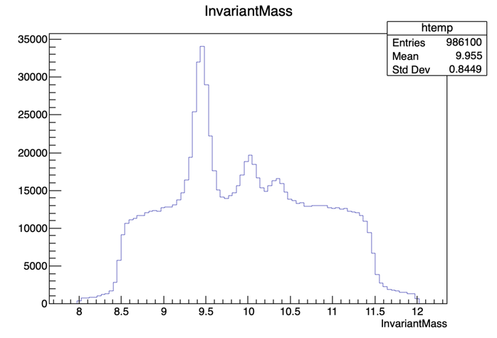
If you got the previous result, we’re ready to go.

The dataset used in this exercise has been collected by the CMS experiment, in proton-proton collisions at the LHC. It contains 986100 entries (muon pair candidates) with an associated invariant mass. For each candidate, the transverse momentum (p_T), rapidity(η) and azimuthal angle (φ) are stored, along with a binary flag PassingProbeTrackingMuon, which is 1 in case the corresponding probe satisfied the tracker muon selection criteria and 0 in case it doesn’t.

Note that it does not really matter what kind of selection criteria these ntuples were created with. The procedure would be the same. You can create your own, similar ntuples with the criteria that you need to study.

As you may have seen, after exploring the content of the root file, the UPSILON_DATA tree has these variables:

InvarianMass

PassingProbeTrackingMuon

ProbeMuon_Pt

ProbeMuon_Eta

ProbeMuon_Phi

We’ll start by calculating the efficiency as a function of p_T. It is useful to have an idea of the distribution of the quantity we want to study. In order to do this, we’ll repeat the steps previously used to plot the invariant mass, but now for the ProbeMuon_Pt variable.

root [] UPSILON_DATA->Draw("ProbeMuon_Pt")

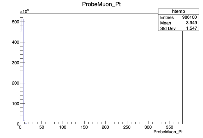
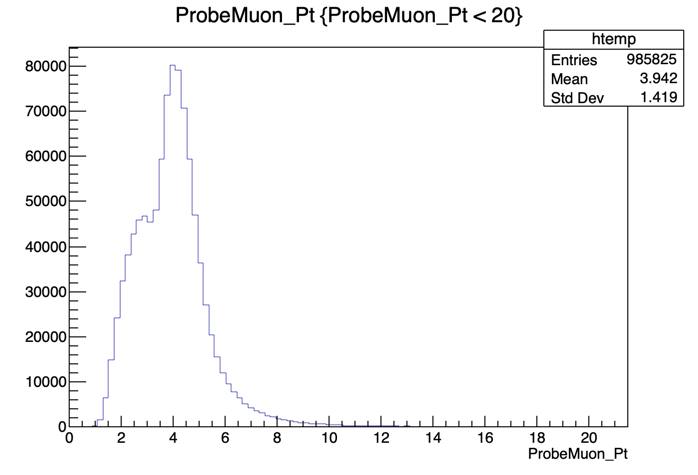
Hmm.. seems like our domain is larger than we need it to be. To fix this, we can apply a constraint to our plot. Try:

root [] UPSILON_DATA->Draw("ProbeMuon_Pt", "ProbeMuon_Pt < 20")

Exit ROOT and get back to the main area:

root [] .q
cd ../../../

Now that you’re acquainted with the data, open the Efficiency.C file. You’ll have to make some small adjustments to the code in this section ( from line:19 to line:32 ):

/*-----------------------------------I N S E R T    C O D E    H E R E-----------------------------------*/
double bins[] =  ...;
int bin_n     =  ...;
 /*------------------------------------------------------------------------------------------------------*/


//Now we must choose initial conditions in order to fit our data
double *init_conditions = new double[4];
/*-----------------------------------I N S E R T    C O D E    H E R E-----------------------------------*/
init_conditions[0] = /*peak1*/;
init_conditions[1] = /*peak2*/;
init_conditions[2] = /*peak3*/;
init_conditions[3] = /*sigma*/;
/*------------------------------------------------------------------------------------------------------*/

We’ll start by choosing the desired bins for the transverse momentum. If you’re feeling brave, choose appropriate bins for our fit remembering that we need a fair amount of data in each bin (more events mean a better fit!). If not, we’ve left a suggestion that you can paste onto the Efficiency.C file. Start with the p_T variable.

Bin Suggestion

double bins[] = {2, 3.4, 4, 4.2, 4.4, 4.7, 5.0, 5.1, 5.2, 5.4, 5.5, 5.6, 5.7, 5.8, 5.9, 6.2, 6.4, 6.6, 6.8, 7.3, 9.5, 13.0, 17.0, 40};
int bin_n = 23;       //-- BINS USED TO CALCULATE PT

double bins[] = {-3, -2.8, -2.6, -2.4, -2.2, -2.0, -1.8, -1.6, -1.4, -1.2, -1.0, -0.8, -0.6, -0.4, -0.2, 0, 0.2, 0.4, 0.5, 0.6, 1.0, 1.2, 1.4, 1.6, 1.8, 2.0, 2.2, 2.4, 2.6, 2.8, 3.0};
int bin_n = 30;       //-- BINS USED TO CALCULATE PHI
   
double bins[] = {-2.0, -1.9, -1.8, -1.7, -1.6, -1.5, -1.4, -1.2, -1.0, -0.8, -0.6, -0.4, 0, 0.2, 0.4, 0.6, 0.7, 0.95, 1.2, 1.4, 1.5, 1.6, 2.0};
int bin_n = 23;       //-- BINS USED TO CALCULATE ETA

Now that the bins are set, we’ll need to define the initial parameters for our fit. You can try to get a good 1st approximation from the plot of the invariant mass that we got before:

or use the suggested values

Suggestion for the Initial Values

Try the following initial values:
init_conditions[0] = 9.46030;
init_conditions[1] = 10.02326;
init_conditions[2] = 10.3552;
init_conditions[3] = 0.08;

We are now ready to execute the fits!

The Fit

We execute a simultaneous fit using a Gaussian curve and a Crystall Ball function for the fist peak (1S) and a gaussian for the remaining peaks. For the background we use a Chebychev polynomial. The function used, doFit(), is implemented in the source file src/DoFit.cpp and it was based on the RooFit library.

You can find generic tutorials for this library here. If you’re starting with RooFit you may also find this one particularly useful.

You won’t need to do anything in src/DoFit.cpp but you can check it out if you’re curious.

Check out `src/DoFit.cpp`

The code here is presented in smaller “digestible” chunks, so it’s easier to understand.

We begin by linking our dataset to a usable object ( the TTree ) and by creating a TCanvas to store the fit plots.

we then define a few RooRealVar and RooFormulaVar objects will be used to select the bin associated to the string condition (i.e. “ProbeMuon_Pt > 10 && ProbeMuon_Pt < 10”). After spliting the original dataset, the resulting two RooDataSet are used to create two binned RooDataHist in which we’ll perform the fits.

double* doFit(string condition, string MuonID_str, string quant, double* init_conditions, bool save = true)
{
    TFile *file0    = TFile::Open("DATA/Upsilon/trackerMuon/T&P_UPSILON_DATA.root");
    TTree *DataTree = (TTree*)file0->Get(("UPSILON_DATA"));

    TCanvas* c_all  = new TCanvas;
    TCanvas* c_pass = new TCanvas;
    
    RooRealVar MuonID(MuonID_str.c_str(), MuonID_str.c_str(), 0, 1); //Muon_Id
    
    RooRealVar InvariantMass("InvariantMass", "InvariantMass", 9, 10.8);
    RooPlot *frame = InvariantMass.frame(RooFit::Title("Invariant Mass"));
    
    double* limits = new double[2];
    if (quant == "Pt") {
        limits[0] = 0;
        limits[1] = 40;
    }
    if (quant == "Eta") {
        limits[0] = -3;
        limits[1] = 3;
    }
    if (quant == "Phi") {
        limits[0] = -2;
        limits[1] = 2;
    }
    RooRealVar quantity(("ProbeMuon_" + quant).c_str(), ("ProbeMuon_" + quant).c_str(), limits[0], limits[1]);
    
    RooFormulaVar* redeuce = new RooFormulaVar("PPTM", condition.c_str(), RooArgList(quantity));
    RooDataSet *Data_ALL    = new RooDataSet("DATA", "DATA", DataTree, RooArgSet(InvariantMass, MuonID, quantity),*redeuce);
    RooFormulaVar* cutvar = new RooFormulaVar("PPTM", (condition + " && " + MuonID_str + " == 1").c_str() , RooArgList(MuonID, quantity));

    RooDataSet *Data_PASSING = new RooDataSet("DATA_PASS", "DATA_PASS", DataTree, RooArgSet(InvariantMass, MuonID, quantity), *cutvar);//

    RooDataHist* dh_ALL     = Data_ALL->binnedClone();
    RooDataHist* dh_PASSING = Data_PASSING->binnedClone();
    

We then create the variables used as parameters in the fit. a0 and a1 used in the Chebychev polynomial (RooChebychev, for the background and sigma, mean1, mean2, mean3 used on the RooCBShape and RooGaussian for the signal. frac1 and frac2 are used as normalization values.

For the yields of the fits, we defined the n_signal and n_background pairs.

    // BACKGROUND VARIABLES
    RooRealVar a0("a0", "a0", 0, -10, 10);
    RooRealVar a1("a1", "a1", 0, -10, 10);

    // BACKGROUND FUNCTION
    RooChebychev background("background","background", InvariantMass, RooArgList(a0,a1));
    
    // GAUSSIAN VARIABLES
    RooRealVar sigma("sigma","sigma",init_conditions[3]);
    RooRealVar mean1("mean1","mean1",init_conditions[0]);
    RooRealVar mean2("mean2","mean2",init_conditions[1]); =(    RooRealVar mean3("mean3","mean3",init_conditions[2]);>.0    // CRYSTAL BALL VARIABLES
    RooRealVar alpha("alpha","alpha", 1.4384e+00); =(    RooRealVar n("n", "n", 1.6474e+01);>.0    // FIT FUNCTIONS
    RooCBShape  gaussian1("signal1","signal1",InvariantMass,mean1,sigma, alpha, n); =(    RooGaussian gaussian2("signal2","signal2",InvariantMass,mean2,sigma);>.0    RooGaussian gaussian3("signal3","signal3",InvariantMass,mean3,sigma);

    RooRealVar frac1("frac1","frac1",7.1345e-01);
    RooRealVar frac2("frac2","frac2",1.9309e-01);    

    double n_signal_initial1 =(Data_ALL->sumEntries(TString::Format("abs(InvariantMass-%g)<0.015",init_conditions[1]))-Data_ALL->sumEntries(TString::Format("abs(InvariantMass-%g)<0.030&&abs(InvariantMass-%g)>.015",init_conditions[1],init_conditions[1]))) / Data_ALL->sumEntries();
    double n_signal_initial2 =(Data_ALL->sumEntries(TString::Format("abs(InvariantMass-%g)<0.015",init_conditions[2]))-Data_ALL->sumEntries(TString::Format("abs(InvariantMass-%g)<0.030&&abs(InvariantMass-%g)>.015",init_conditions[2],init_conditions[2]))) / Data_ALL->sumEntries();
    double n_signal_initial3 =(Data_ALL->sumEntries(TString::Format("abs(InvariantMass-%g)<0.015",init_conditions[3]))-Data_ALL->sumEntries(TString::Format("abs(InvariantMass-%g)<0.030&&abs(InvariantMass-%g)>.015",init_conditions[3],init_conditions[3]))) / Data_ALL->sumEntries();
    
    double n_signal_initial_total = n_signal_initial1 + n_signal_initial2 + n_signal_initial3;
    
    double n_back_initial = 1. - n_signal_initial1 - n_signal_initial2 -n_signal_initial3;
    
    RooRealVar n_signal_total("n_signal_total","n_signal_total",n_signal_initial_total,0.,Data_ALL->sumEntries());
    RooRealVar n_signal_total_pass("n_signal_total_pass","n_signal_total_pass",n_signal_initial_total,0.,Data_PASSING->sumEntries());
    
    RooRealVar n_back("n_back","n_back",n_back_initial,0.,Data_ALL->sumEntries());
    RooRealVar n_back_pass("n_back_pass","n_back_pass",n_back_initial,0.,Data_PASSING->sumEntries());

After defining the individual pdfs that will be used in the fit, we add them together to make our model with the signal and background. We then combine the data onto a RooSimultaneous so that we can execute a simultaneous fit with the fitTo method. The fit result is then stored.

    RooAddPdf* signal;
    RooAddPdf* model;
    RooAddPdf* model_pass;
    
    signal     = new RooAddPdf("signal", "signal", RooArgList(gaussian1, gaussian2,gaussian3), RooArgList(frac1, frac2));
    model      = new RooAddPdf("model","model", RooArgList(*signal, background),RooArgList(n_signal_total, n_back));
    model_pass = new RooAddPdf("model_pass", "model_pass", RooArgList(*signal, background),RooArgList(n_signal_total_pass, n_back_pass));
    
    // SIMULTANEOUS FIT
    RooCategory sample("sample","sample") ;
    sample.defineType("All") ;
    sample.defineType("PASSING") ;
    
    RooDataHist combData("combData","combined data",InvariantMass,Index(sample),Import("ALL",*dh_ALL),Import("PASSING",*dh_PASSING));
    
    RooSimultaneous simPdf("simPdf","simultaneous pdf",sample) ;
    
    simPdf.addPdf(*model,"ALL");
    simPdf.addPdf(*model_pass,"PASSING");
    
    RooFitResult* fitres = new RooFitResult;
    fitres = simPdf.fitTo(combData, RooFit::Save());

    // OUTPUT ARRAY
    double* output = new double[4];
    
    RooRealVar* yield_ALL = (RooRealVar*) fitres->floatParsFinal().find("n_signal_total");
    RooRealVar* yield_PASS = (RooRealVar*) fitres->floatParsFinal().find("n_signal_total_pass");
    
    output[0] = yield_ALL->getVal();
    output[1] = yield_PASS->getVal();
    
    output[2] = yield_ALL->getError();
    output[3] = yield_PASS->getError();

The rest of the code has to do with the plotting of the fit and with memory management.

    frame->SetTitle("ALL");
    frame->SetXTitle("#mu^{+}#mu^{-} invariant mass [GeV/c^{2}]");
    Data_ALL->plotOn(frame);
    
    model->plotOn(frame);
    model->plotOn(frame,RooFit::Components("signal1"),RooFit::LineStyle(kDashed),RooFit::LineColor(kGreen));
    model->plotOn(frame,RooFit::Components("signal2"),RooFit::LineStyle(kDashed),RooFit::LineColor(kMagenta - 5));
    model->plotOn(frame,RooFit::Components("signal3"),RooFit::LineStyle(kDashed),RooFit::LineColor(kOrange));
    model->plotOn(frame,RooFit::Components("background"),RooFit::LineStyle(kDashed),RooFit::LineColor(kRed));
    
    c_all->cd();
    frame->Draw("");
    
    RooPlot *frame_pass = InvariantMass.frame(RooFit::Title("Invariant Mass"));
    
    c_pass->cd();
    
    frame_pass->SetTitle("PASSING");
    frame_pass->SetXTitle("#mu^{+}#mu^{-} invariant mass [GeV/c^{2}]");
    Data_PASSING->plotOn(frame_pass);
    
    model_pass->plotOn(frame_pass);
    model_pass->plotOn(frame_pass,RooFit::Components("signal1"),RooFit::LineStyle(kDashed),RooFit::LineColor(kGreen));
    model_pass->plotOn(frame_pass,RooFit::Components("signal2"),RooFit::LineStyle(kDashed),RooFit::LineColor(kMagenta - 5));
    model_pass->plotOn(frame_pass,RooFit::Components("signal3"),RooFit::LineStyle(kDashed),RooFit::LineColor(kOrange));
    model_pass->plotOn(frame_pass,RooFit::Components("background"),RooFit::LineStyle(kDashed),RooFit::LineColor(kRed));
    
    frame_pass->Draw();

    if(save)
    {
        c_pass->SaveAs(("Fit Result/" + condition + "_ALL.pdf").c_str());
        c_all->SaveAs (("Fit Result/" + condition + "_PASS.pdf").c_str());
    }
        
    // DELETING ALLOCATED MEMORY
    delete[] limits;
    //
    delete file0;
    //
    delete Data_ALL;
    delete Data_PASSING;
    //
    delete dh_ALL;
    delete dh_PASSING;
    //
    delete cutvar;
    delete redeuce;
    //
    delete signal;
    //
    delete c_all;
    delete c_pass;
    //
    delete model;
    delete model_pass;
   delete fitres;
   
   return output;
}

The fitting and storing of the fit output of each bin is achieved by the following loop in the Efficiency.C code.

for (int i = 0; i < bin_n; i++)
{
    if (DataIsMC)
        yields_n_errs[i] = McYield(conditions[i]);
    else
        yields_n_errs[i] = doFit(conditions[i], "PassingProbeTrackerMuon", init_conditions);
}

The McYield() function (src/McYield.cpp) has the same output as doFit() and has to do with Monte Carlo dataset, which only contains signal for the 1S peak.

To get the efficiency plot, we used the TEfficiency class from ROOT. You’ll see that in order to create a TEfficiency object, one of the constructors requires two TH1 objects, i.e., two histograms. One with all the probes and one with the passing probes.

The creation of these TH1 objects is taken care of by the src/make_hist.cpp code.

Check out `src/make_hist.cpp`

TH1F* make_hist(string name, double** values, int qnt, int bin_n, Double_t* binning, bool IsDataMc, bool DRAW = false)
{
   //AddBinContent
   //HISTOGRAM NEEDS TO HAVE VARIABLE BINS
  
   TH1F* hist = new TH1F(name.c_str(), name.c_str(), bin_n, binning);

   for (int i = 0; i < bin_n; i++)
   {
       hist->SetBinContent(i, values[i][qnt]);
       if (IsDataMc == false)
           hist->SetBinError(i, values[i][qnt+2]);
   }
   if (DRAW)
   {
       TCanvas* xperiment = new TCanvas;
       xperiment->cd();
       hist->Draw();
   }
   return hist;
}

To plot the efficiency we used the src/get_efficiency.cpp function.

Check out `get_efficiency.cpp`

TEfficiency* get_efficiency(TH1F* ALL, TH1F* PASS)ID_str, double* init_conditions, bool save = TRUE) // RETURNS ARRAY WITH [yield_all, yield_pass, err_all, err_pass]    ->   OUTPUT ARRAY
{
   TFile* pFile = new TFile("Efficiency_Run2011.root","recreate");lues, int qnt, int bin_n, Double_t* binning, bool IsDataMc, bool DRAW = FALSE)
   TEfficiency* pEff = new TEfficiency();
   pEff->SetName("Efficiency");name.c_str(), bin_n, binning);

   pEff->SetPassedHistogram(*PASS, "f");
   pEff->SetTotalHistogram (*ALL,"f");
   [qnt]);
   pEff->SetDirectory(gDirectory);
   pFile->Write();i][qnt+2]);
   
   TCanvas* oi = new TCanvas();
   oi->cd();
   pEff->Draw();;
   
   gPad->Update();

   //Set range in y axis

   auto graph = pEff->GetPaintedGraph();
   graph->SetMinimum(0.8);
   graph->SetMaximum(1.2);
   gPad->Update();
 
   return pEff;
}

Note that we load all these functions in the src area directly in header of the Efficiency.C code.

Now that you understand what the Efficiency.C macro does, run your code with in a batch mode (-b) and with a quit-when-done switch (-q):

root -q -b Efficiency.C

When the execution finishes, you should have 2 new files. One on your working directory: Histograms.root, and another one Efficiency_Run2011.root located at /Efficiency Result/Pt. The second contains the efficiency we calculated! the first file is used to redo any unusable fits. To open Efficiency_Run2011.root, on your working directory type:

root -l
new TBrowser

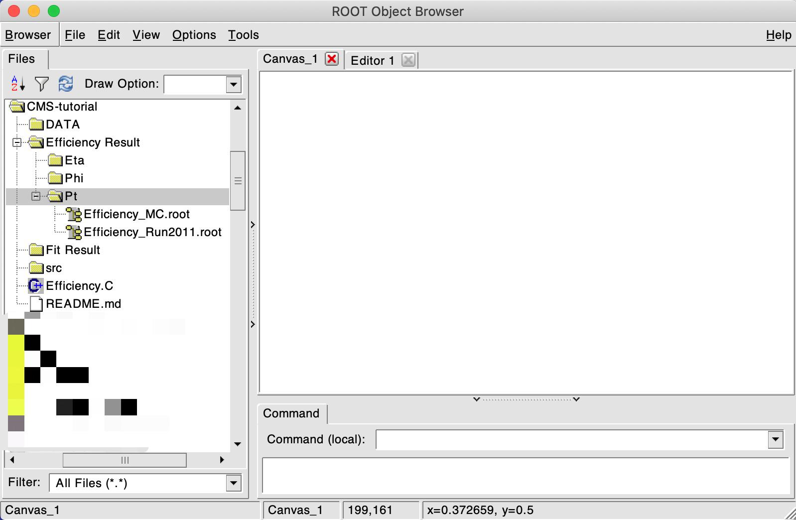
A window like this should have popped up. If you click on Efficiency_Run2011.root, a plot will show up with the efficiency value for each bin!

If you want, check out the PDF files under the Fit\ Result/ directory, which contain the fitting results.

Now we must re-run the code, but before that, change DataIsMc value to TRUE. This will generate an efficiency for the simulated data, so that we can compare it with the 2011 run.

Check that you have both Efficiency_Run2011.root and Efficiency_MC.root files in the following directory Efficiency Result/Pt.

If so, now uncomment Efficiency.C line: 66:

//  compare_efficiency(quantity, "Efficiency_Result/Pt/Efficiency_Run2011.root", "Efficiency_Result/Pt/Efficiency_MC.root");

and run the macro again. You should get something like the following result if you inspect the image at Comparison\ Run2011\ vs\ MC/Efficiency.png.

If everything went well and you still have time to go, repeat this process for the two other variables, η and φ!

In case you want to change one of the fit results, use the change_bin.cpp function commented on line:61.

Important note!

Don’t forget to comment line:68 when repeating the procedure for the other quantities!
compare_efficiency(quantity, "Efficiency Result/" + quantity + "/Efficiency_MC.root", "Efficiency Result/" + quantity + "/Efficiency_Run2011.root");

Extra challenge

Fancy some more work? Download this J/ψ dataset and try out the new methods you just learned! You’ll have to change the DoFit.cpp function since J/ψ’s only peak is made up of a Crystall ball and a Gaussian curve. Good luck!

Key Points

The dataset for this tutorial contemplates one Muon Id (Tracker Muon) and further contains the three kinematic variables (p_T, η, φ)

Everything in this tutorial should be done using only the Efficiency.C file. The check out sections are only for you to see what’s going on under the hood

Documentation available here

Sideband subtraction method

Overview

Teaching: 5 min
Exercises: 35 min

Questions

What is the sideband subtraction method?

How to implement it?

Objectives

Learn how to set bins in a sideband subtraction tool.

Get efficiency by using the sideband subtraction on real data and simulation.

Signal extraction: sideband subtraction method

The reconstruction efficiency is calculated using only signal muons. In order to measure the efficiency, we need a way to extract signal from the dataset. You’ve used the fitting method and now you’ll meet the sideband subtraction method.

This method consists in choosing sideband and signal regions in invariant mass distribution. The sideband regions (shaded in red in the figure) have background particles and the signal region (shared in green in the figure) has background and signal particles.

Invariant Mass histogram

Note: The background corresponds to candidates that do not correspond to the decay of a genuine resonance; for example, the pair is formed by the tag muon associated to an uncorrelated track produced elsewhere in the collision; the corresponding invariant mass has thus a smooth continuous shape, that is extrapolated from the signal regions into the sideband region.

Note: we choose only the ϒ (1S) signal for selecting the signal region; simulation information is further available for this resonance, allowing in the end for a comparison of results, between data and simulation.

For each event category (i.e. Pass and All), and for a given variable of interest (e.g., the probe pT), two distributions are obtained, one for each region (Signal and Sideband). In order to obtain the variable distribution for the signal only, we proceed by subtracting the Background distribution (Sideband region) from the Signal+Background one (Signal region):

Sideband Subtraction equation

Where the normalization α factor quantifies the quantity of background present in the signal region>

Alpha factor equation

And for the uncertainty:

Sideband Subtraction errors equation

Applying those equations we get histograms like this:

Invariant Mass histogram

Solid blue line (Total) = particles in signal region;
Dashed blue line (Background) = particles in sideband regions;
Solid magenta line (signal) = signal histogram (background subtracted).

You will see this histogram on this exercise.

About this code

More info about this code can be found here.

Preparing files

First, we need to get the code. Go to folder you have created for this lesson and on your terminal type:

git clone -b sideband git://github.com/allanjales/efficiency_tagandprobe
cd efficiency_tagandprobe

To copy the ϒ dataset from real data file to your machine (requires 441 MB), type:

wget --load-cookies /tmp/cookies.txt "https://docs.google.com/uc?export=download&confirm=$(wget --quiet --save-cookies /tmp/cookies.txt --keep-session-cookies --no-check-certificate 'https://docs.google.com/uc?export=download&id=1Fj-rrKts8jSSMdwvOnvux68ydZcKB521' -O- | sed -rn 's/.*confirm=([0-9A-Za-z_]+).*/\1\n/p')&id=1Fj-rrKts8jSSMdwvOnvux68ydZcKB521" -O Run2011A_MuOnia_Upsilon.root && rm -rf /tmp/cookies.txt

This code downloads the file directly from Google Drive.

Run this code to download the simulation ntuple for ϒ (requires 66 MB):

wget --load-cookies /tmp/cookies.txt "https://docs.google.com/uc?export=download&confirm=$(wget --quiet --save-cookies /tmp/cookies.txt --keep-session-cookies --no-check-certificate 'https://docs.google.com/uc?export=download&id=1ZzAOOLCKmCz0Q6pVi3AAiYFGKEpP2efM' -O- | sed -rn 's/.*confirm=([0-9A-Za-z_]+).*/\1\n/p')&id=1ZzAOOLCKmCz0Q6pVi3AAiYFGKEpP2efM" -O Upsilon1SToMuMu_MC_full.root && rm -rf /tmp/cookies.txt

Now, check if everything is ok:

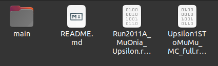
ls

main  README.md  Run2011A_MuOnia_Upsilon.root  Upsilon1SToMuMu_MC_full.root

Your efficiency_tagandprobe folder should have these files:

Files in efficiency_tagandprobe folder

Preparing code for Data

I will teach you to manage the files on the terminal, but you can use a graphical file explorer.

We need to edit some settings. Open settings.cpp:

cd main/config
ls

cuts.h  settings.cpp

There are different ways to open this file. You can try to run:

gedit settings.cpp

Or, if you can not use gedit, try nano:

nano settings.cpp

“I do not have nano!”

You can try to use any text editor, but here is some commands you cant try to use to install it:

Ubuntu/Debian: sudo apt-get -y install nano.

RedHat/CentOS/Fedora: sudo yum install nano.

Mac OS X: nano is installed by default.

We want to calculate efficiencies of tracker muons. With the settings.cpp file opened, make sure to let the variables like this:

//Canvas drawing
bool shouldDrawInvariantMassCanvas       = true;
bool shouldDrawInvariantMassCanvasRegion = true;
bool shouldDrawQuantitiesCanvas          = true;
bool shouldDrawEfficiencyCanvas          = true;

//Muon id analyse	
bool doTracker    = true;
bool doStandalone = false;
bool doGlobal     = false;

We want to calculate the efficiency using specific files that we downloaded. They name are Run2011A_MuOnia_Upsilon.root and Upsilon1SToMuMu_MC_full.root and are listed in const char *files[]. While settings.cpp is open, try to use the variable int useFile to run Run2011A_MuOnia_Upsilon.root.

How to do this

Make sure useFile is correct:

//List of files
const char *files[] = {"../data_histoall.root",
                       "../Run2011AMuOnia_mergeNtuple.root",""
                       "../JPsiToMuMu_mergeMCNtuple.root",
                       "../Run2011A_MuOnia_Upsilon.root",
                       "../Upsilon1SToMuMu_MC_full.root"};

const char* directoriesToSave[] = {"../results/result/",
                                   "../results/Jpsi Run 2011/",
                                   "../results/Jpsi MC 2020/",
                                   "../results/Upsilon Run 2011/",
                                   "../results/Upsilon MC 2020/"};


//MAIN OPTIONS

//Which file of files (variable above) should use
int useFile = 3;

It will tell which configuration the program will use. So, the macro will run with the ntuple in files[useFile] and the results will be stored in directoriesToSave[useFile].

the first three files won’t be used in this execise.

About code

Normally we need to set the variables bool isMC and const char* resonance, but at this time it is already done and set automatically for these ntuples’ names.

Editting bins

The code allows to define the binning of the kinematic variable, to ensure each bin is sufficiently populated, for increased robustness. To change the binning, locate PassingFailing.h

cd ../classes
ls

FitFunctions.h   MassValues.h      PtEtaPhi.h             TagProbe.h
InvariantMass.h  PassingFailing.h  SidebandSubtraction.h  Type.h

And then Open PassingFailing.h

gedit PassingFailing.h

Search for the createEfficiencyPlot(...) function. You’ll find something like this:

void createHistogram(TH1D* &histo, const char* histoName)
{...}

For each quantity (pT, eta, phi) we used different bins. To change the bins, look inside the createEfficiencyPlot(...) function. In a simpler version, you’ll see a structure like this:

//Variable bin for pT
if (strcmp(quantityName, "Pt") == 0)
{
	//Here creates histogram for pT
}

//Variable bin for eta
else if (strcmp(quantityName, "Eta") == 0)
{
	//Here creates histogram for eta
}

//Bins for phi
else
{
	//Here creates histogram for phi
}

See the whole scructure

Don’t be scared! Code doens’t bite.

//Variable bin for pT
if (strcmp(quantityName, "Pt") == 0)
{
	double xbins[10000];
	xbins[0] = .0;
	int nbins = 0;
	double binWidth = 1.;
	for (int i = 1; xbins[i-1] < xMax+binWidth; i++)
	{
		xbins[i] = xbins[i-1] < 1. ? 1. : xbins[i-1] *(1+binWidth);
		nbins++;
	}

	histo = new TH1D(hName.data(), hTitle.data(), nbins, xbins);
}

//Variable bin for eta
else if (strcmp(quantityName, "Eta") == 0)
{
	double xbins[10000];
	xbins[0] = .5;
	int nbins = 0;
	double binWidth = 0.2;

	//For positive
	for (int i = 1; xbins[i-1] < xMax+binWidth; i++)
	{
		xbins[i] = xbins[i-1] < 1. ? 1. : xbins[i-1] *(1+binWidth);
		nbins++;
	}

	//Duplicate array and create another
	double rxbins[nbins*2+1];
	int entry = 0;
	for (int i = nbins; i >= 0; i--)
	{
		rxbins[entry] = -xbins[i];
		entry++;
	}
	rxbins[entry] = 0.;
	entry++;
	for (int i = 0; i <= nbins; i++)
	{
		rxbins[entry] = xbins[i];
		entry++;
	}
	
	histo = new TH1D(hName.data(), hTitle.data(), entry-1, rxbins);
}

//Bins for phi 
else
{
	if (strcmp(quantityUnit, "") == 0)
	{
		yAxisTitleForm += " / (%1." + to_string(decimals) + "f)";
	}
	else
	{
		yAxisTitleForm += " / (%1." + to_string(decimals) + "f " + string(quantityUnit) + ")";
	}

 histo = new TH1D(hName.data(), hTitle.data(), nBins, xMin, xMax);
} 

The code that creates the histogram bins is located inside the conditionals and is commented. You can edit this code and uncomment to create histogram bins however you want. Instead of using a function to generate the bins, we can also define them manually.

As we intend to compare the results between data and simulation, but also between the sideband and fitting methods, you are advised to employ the same bin choice. Change your the code to this:

//Variable bin for pT
if (strcmp(quantityName, "Pt") == 0)
{
	double xbins[] = {2., 3.4, 4, 4.2, 4.4, 4.7, 5.0, 5.1, 5.2, 5.4, 5.5, 5.6, 5.7, 5.8, 5.9, 6.2, 6.4, 6.6, 6.8, 7.3, 9.5, 13.0, 17.0, 40.};
	int nbins = 23;

	histo = new TH1D(hName.data(), hTitle.data(), nbins, xbins);
}

//Variable bin for eta
else if (strcmp(quantityName, "Eta") == 0)
{
	double xbins[] = {-2.0, -1.9, -1.8, -1.7, -1.6, -1.5, -1.4, -1.2, -1.0, -0.8, -0.6, -0.4, 0, 0.2, 0.4, 0.6, 0.7, 0.95, 1.2, 1.4, 1.5, 1.6, 2.0};
	int nbins = 22;

	histo = new TH1D(hName.data(), hTitle.data(), nbins, xbins);
}

//Bins for phi
else
{
	double xbins[] =  {-3, -2.8, -2.6, -2.4, -2.2, -2.0, -1.8, -1.6, -1.4, -1.2, -1.0, -0.8, -0.6, -0.4, -0.2, 0, 0.2, 0.4, 0.5, 0.6, 1.0, 1.2, 1.4, 1.6, 1.8, 2.0, 2.2, 2.4, 2.6, 2.8, 3.0};
	int nbins = 30;

	histo = new TH1D(hName.data(), hTitle.data(), nbins, xbins);
}

Running the code

After setting the configurations, it’s time to run the code. Go back to the main directory and make sure macro.cpp is there.

cd ..
ls

classes  compare_efficiency.cpp  config  macro.cpp

Run the macro.cpp:

root -l -b -q macro.cpp

"../results/Upsilon Run 2011/" directory created OK
Using "../Run2011A_MuOnia_Upsilon.root" ntuple
resonance: Upsilon
Using method 2
Data analysed = 986100 of 986100

In this process, more informations will be printed in terminal while plots will be created on specified (these plots are been saved in a folder). The message below tells you that code has finished running:

Done. All result files can be found at "../results/Upsilon_Run_2011/"

Common errors

If you run the code and your terminal printed some erros like:
Error in <ROOT::Math::Cephes::incbi>: Wrong domain for parameter b (must be > 0)
This occurs when the contents of a bin of the pass histogram is greater than the corresponding bin in the total histogram. With sideband subtraction, depending on bins you choose, this can happen and will result in enormous error bars.

This issue may be avoided by fine-tuning the binning choice. For now, these messages may be ignored.

Probe Efficiency results for Data

If all went well, your results are going to be like these:

Efficiency plot

Preparing and running the code for simulation

Challenge

Try to run the same code on the Upsilon1SToMuMu_MC_full.root file we downloaded.
Tip

You will need the redo the steps above, setting:
int useFile = 4;
in main/config/settings.cpp file.

Comparison between real data and simulation

We’ll do this in the last section of this exercise. So the challenge above is mandatory.

Extra challenge

If you are looking for an extra exercise, you can try to apply the same logic, changing some variables you saw, in order to get results for the J/ψ nutpple.

To download the J/ψ real data ntupple (requires 3.3 GB):
wget --load-cookies /tmp/cookies.txt "https://docs.google.com/uc?export=download&confirm=$(wget --quiet --save-cookies /tmp/cookies.txt --keep-session-cookies --no-check-certificate 'https://docs.google.com/uc?export=download&id=16OqVrHIB4wn_5X8GEZ3NxnAycZ2ItemZ' -O- | sed -rn 's/.*confirm=([0-9A-Za-z_]+).*/\1\n/p')&id=16OqVrHIB4wn_5X8GEZ3NxnAycZ2ItemZ" -O Run2011AMuOnia_mergeNtuple.root && rm -rf /tmp/cookies.txt
To download the J/ψ simulated data ntuple (requires 515 MB):
wget --load-cookies /tmp/cookies.txt "https://docs.google.com/uc?export=download&confirm=$(wget --quiet --save-cookies /tmp/cookies.txt --keep-session-cookies --no-check-certificate 'https://docs.google.com/uc?export=download&id=1dKLJ5RIGrBp5aIJrvOQw5lWLQSHUgEnf' -O- | sed -rn 's/.*confirm=([0-9A-Za-z_]+).*/\1\n/p')&id=1dKLJ5RIGrBp5aIJrvOQw5lWLQSHUgEnf" -O JPsiToMuMu_mergeMCNtuple.root && rm -rf /tmp/cookies.txt
As this dataset is larger, the code will run slowly. It can take several minutes to be completed depending where the code is been running

Key Points

There is a file in main/config/settings.cpp where you can edit some options.

You can edit the binnig in the main/classes/PassingFailing.h file.

The main code is located in main/macro.cpp

Results comparison

Overview

Teaching: 5 min
Exercises: 20 min

Questions

How good are the results?

Objectives

Compare efficiencies between real data and simulations.

Compare efficiencies between sideband subtraction and fitting methods.

How sideband subtraction method code stores its files

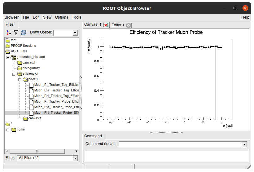
the Sideband subtraction code saves every efficiency plot in efficiency/plots/ folder inside a single generated_hist.root file. Lets check it!

You’re probably on the main directory. Lets go back a directory.

cd ..
ls

main  README.md  results  Run2011A_MuOnia_Upsilon.root  Upsilon1SToMuMu_MC_full.root

A folder named results showed up on this folder. Lets go check its content.

cd results
ls

Comparison_Upsilon_Sideband_Run_vs_MC  Upsilon_MC_2020  Upsilon_Run_2011

If you did every step of the sideband subtraction on this page lesson, these results should match with the results on your pc. Access one of those folders (except comparison).

cd Upsilon_Run_2011
ls

Efficiency_Tracker_Probe_Eta.png  Tracker_Probe_Phi_All.png
Efficiency_Tracker_Probe_Phi.png  Tracker_Probe_Phi_Passing.png
Efficiency_Tracker_Probe_Pt.png   Tracker_Probe_Pt_All.png
Efficiency_Tracker_Tag_Eta.png    Tracker_Probe_Pt_Passing.png
Efficiency_Tracker_Tag_Phi.png    Tracker_Tag_Eta_All.png
Efficiency_Tracker_Tag_Pt.png     Tracker_Tag_Eta_Passing.png
generated_hist.root               Tracker_Tag_Phi_All.png
InvariantMass_Tracker.png         Tracker_Tag_Phi_Passing.png
InvariantMass_Tracker_region.png  Tracker_Tag_Pt_All.png
Tracker_Probe_Eta_All.png         Tracker_Tag_Pt_Passing.png
Tracker_Probe_Eta_Passing.png

Here, all the output plots you saw when running the sideband subtraction method are stored as a .png. Aside from them, there’s a generated_hist.root that stores the efficiency in a way that we can manipulate it after. This file is needed to run the comparison between efficiencies for the sideband subtraction method. Lets look inside of this file.

Run this command to open generated_hist.root with ROOT:

root -l generated_hist.root

root [0] 
Attaching file generated_hist.root as _file0...
(TFile *) 0x55dca0f04c50
root [1]

Lets check its content. Type on terminal:

new TBrowser

You should see something like this:

Invariant Mass histogram

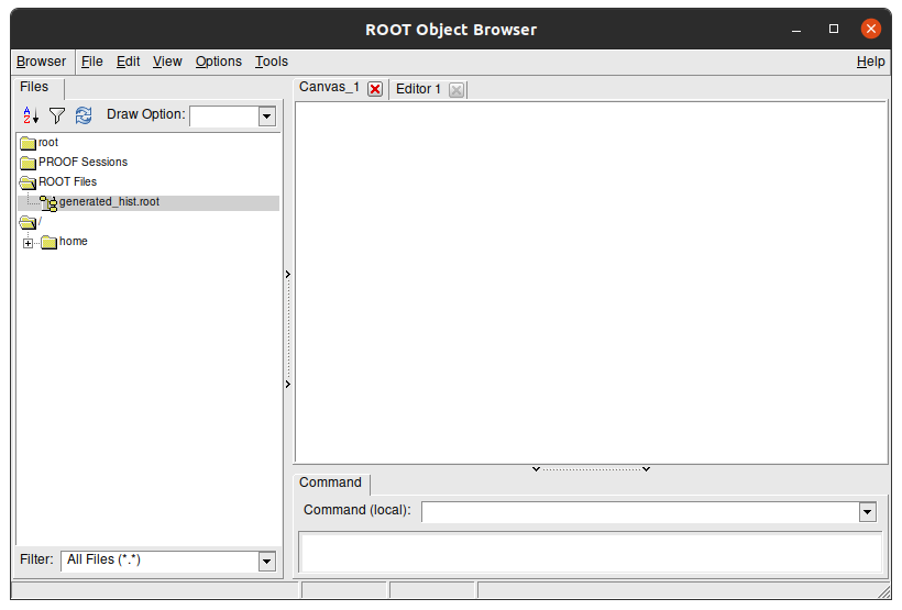
This is a visual navigator of a .root file. Here you can see the struture of generated_hist.root. Double click the folders to open them and see their content. The Efficiency plots we see are stored in efficiency/plots/ folder:

Invariant Mass histogram

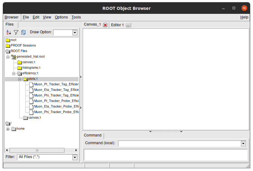
You can double click each plot to see its content:

Invariant Mass histogram

Tip

To close this window, click on terminal and press Ctrl + C. This command stops any processes happening in the terminal.

Key Point

As you see, the .root file has a path inside and the efficiencies plots have paths inside them as well!

Comparison results between real data and simulations for sideband method

After runinng the sideband subtraction code, we get a .root with all the efficiencies plots inside it in two different folders:

../results/Upsilon_Run_2011/generated_hist.root
../results/Upsilon_MC_2020/generated_hist.root

We’ll get back to this on the discussion below.

Head back to the main folder. Inside of it there is a code for the efficiency plot comparison. Lets check it out.

cd main
ls

classes  compare_efficiency.cpp  config  macro.cpp

There is it. Now lets open it.

gedit compare_efficiency.cpp

Its easy to prepare it for the sideband subtraction comparison. Our main editing point can be found in this part:

int useScheme = 0;
//Upsilon Sideband Run vs Upsilon Sideband MC
//Upsilon Fitting  Run vs Upsilon Fitting  MC
//Upsilon Sideband Run vs Upsilon Fitting  Run

//Root files and paths for Tefficiency objects inside these files
const char* filePathsEff0[][2] = {
	{"../results/Upsilon_Run_2011/generated_hist.root", "efficiency/plots/Muon_Pt_Tracker_Probe_Efficiency"},
	{"../results/Upsilon_Run_2011/generated_hist.root", "efficiency/plots/Muon_Eta_Tracker_Probe_Efficiency"},
	{"../results/Upsilon_Run_2011/generated_hist.root", "efficiency/plots/Muon_Phi_Tracker_Probe_Efficiency"},
	{"../results/Upsilon_Run_2011/generated_hist.root", "efficiency/plots/Muon_Pt_Standalone_Probe_Efficiency"},
	{"../results/Upsilon_Run_2011/generated_hist.root", "efficiency/plots/Muon_Eta_Standalone_Probe_Efficiency"},
	{"../results/Upsilon_Run_2011/generated_hist.root", "efficiency/plots/Muon_Phi_Standalone_Probe_Efficiency"},
	{"../results/Upsilon_Run_2011/generated_hist.root", "efficiency/plots/Muon_Pt_Global_Probe_Efficiency"},
	{"../results/Upsilon_Run_2011/generated_hist.root", "efficiency/plots/Muon_Eta_Global_Probe_Efficiency"},
	{"../results/Upsilon_Run_2011/generated_hist.root", "efficiency/plots/Muon_Phi_Global_Probe_Efficiency"}
};

//Root files and paths for Tefficiency objects inside these files
const char* filePathsEff1[][2] = {
	{"../results/Upsilon_MC_2020/generated_hist.root", "efficiency/plots/Muon_Pt_Tracker_Probe_Efficiency"},
	{"../results/Upsilon_MC_2020/generated_hist.root", "efficiency/plots/Muon_Eta_Tracker_Probe_Efficiency"},
	{"../results/Upsilon_MC_2020/generated_hist.root", "efficiency/plots/Muon_Phi_Tracker_Probe_Efficiency"},
	{"../results/Upsilon_MC_2020/generated_hist.root", "efficiency/plots/Muon_Pt_Standalone_Probe_Efficiency"},
	{"../results/Upsilon_MC_2020/generated_hist.root", "efficiency/plots/Muon_Eta_Standalone_Probe_Efficiency"},
	{"../results/Upsilon_MC_2020/generated_hist.root", "efficiency/plots/Muon_Phi_Standalone_Probe_Efficiency"},
	{"../results/Upsilon_MC_2020/generated_hist.root", "efficiency/plots/Muon_Pt_Global_Probe_Efficiency"},
	{"../results/Upsilon_MC_2020/generated_hist.root", "efficiency/plots/Muon_Eta_Global_Probe_Efficiency"},
	{"../results/Upsilon_MC_2020/generated_hist.root", "efficiency/plots/Muon_Phi_Global_Probe_Efficiency"}
};

//How comparisons will be saved
const char* resultNames[] = {
	"Muon_Pt_Tracker_Probe_Efficiency.png",
	"Muon_Eta_Tracker_Probe_Efficiency.png",
	"Muon_Phi_Tracker_Probe_Efficiency.png",
	"Muon_Pt_Standalone_Probe_Efficiency.png",
	"Muon_Eta_Standalone_Probe_Efficiency.png",
	"Muon_Phi_Standalone_Probe_Efficiency.png",
	"Muon_Pt_Global_Probe_Efficiency.png",
	"Muon_Eta_Global_Probe_Efficiency.png",
	"Muon_Phi_Global_Probe_Efficiency.png"
};

In the scope above we see:

int useScheme represents which comparison you are doing.

const char* filePathsEff0 is an array with location of the first plots.

const char* filePathsEff1 is an array with location of the second plots.

const char resultNames is an array with names which comparison will be saved.

Plots in const char* filePathsEff0[i] will be compared with plots in const char* filePathsEff1[i]. The result will be saved as const char* resultNames[i].

Everything is uptodate to compare sideband subtraction’s results between real data and simulations, except it is comparing standalone and global muons. As we are looking for tracker muons efficiencies only, you should delete lines with Standalone and Global words

See result scructure

If you deleted the right lines, your code now should be like this:

int useScheme = 0;
//Upsilon Sideband Run vs Upsilon Sideband MC
//Upsilon Fitting  Run vs Upsilon Fitting  MC
//Upsilon Sideband Run vs Upsilon Fitting  Run

//Root files and paths for Tefficiency objects inside these files
const char* filePathsEff0[][2] = {
	{"../results/Upsilon_Run_2011/generated_hist.root", "efficiency/plots/Muon_Pt_Tracker_Probe_Efficiency"},
	{"../results/Upsilon_Run_2011/generated_hist.root", "efficiency/plots/Muon_Eta_Tracker_Probe_Efficiency"},
	{"../results/Upsilon_Run_2011/generated_hist.root", "efficiency/plots/Muon_Phi_Tracker_Probe_Efficiency"}
};

//Root files and paths for Tefficiency objects inside these files
const char* filePathsEff1[][2] = {
	{"../results/Upsilon_MC_2020/generated_hist.root", "efficiency/plots/Muon_Pt_Tracker_Probe_Efficiency"},
	{"../results/Upsilon_MC_2020/generated_hist.root", "efficiency/plots/Muon_Eta_Tracker_Probe_Efficiency"},
	{"../results/Upsilon_MC_2020/generated_hist.root", "efficiency/plots/Muon_Phi_Tracker_Probe_Efficiency"}
};

//How comparisons will be saved
const char* resultNames[] = {
	"Muon_Pt_Tracker_Probe_Efficiency.png",
	"Muon_Eta_Tracker_Probe_Efficiency.png",
	"Muon_Phi_Tracker_Probe_Efficiency.png"
};

Let your variables like this.

Now you need to run the code. To do this, save the file and type on your terminal:

root -l compare_efficiency.cpp

If everything went well, the message you’ll see in terminal at end of the process is:

Use Scheme: 0
Done. All result files can be found at "../results/Comparison_Upsilon_Sideband_Run_vs_MC/"

Note

The command above to run the code will display three new windows on your screen with comparison plots. You can avoid them by running straight the command below.
root -l -b -q compare_efficiency.cpp
In this case, to check it results you are going to need go for result folder (printed on code run) and check images there by yourself. You can try to run TBrowser again:
cd [FOLDER_PATH]
root -l
new TBrowser

And as output plots comparsion, you get:

Invariant Mass histogram

Now you can type the command below to quit root and close all created windows:

.q

How fitting method code stores its files

To do the next part, first you need to understand how the fitting method code saves its files in a different way to the sideband subtraction method code. Lets look at how they are saved.

If you look inside CMS-tutorial\Efficiency Result\ folder, where is stored fitting method results, you will see another folder named trackerMuon. Inside of it you’ll see:

Invariant Mass histogram

Inside of them, there are two files:

Invariant Mass histogram

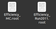
If you go with your terminal to this folder and run this command, you’ll see that the result files only have one plot.\

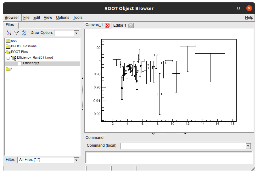
root -l Efficiency_Run2011.root

root [0] 
Attaching file Efficiency_Run2011.root as _file0...
(TFile *) 0x55f7152a8970
root [1]

Now lets look at its content. Type on terminal:

new TBrowser

It has only one plot, because the others are in different files.

Invariant Mass histogram

Key Point

There is a .root file for each efficiency plot created with the fitting method.

Comparison results between real data and simulations for fitting method

Go back to the main folder.

cd main
ls

classes  compare_efficiency.cpp  config  macro.cpp

Open compare_efficiency.cpp again

gedit compare_efficiency.cpp

This is how your code should look like now:

int useScheme = 0;
//Upsilon Sideband Run vs Upsilon Sideband MC
//Upsilon Fitting  Run vs Upsilon Fitting  MC
//Upsilon Sideband Run vs Upsilon Fitting  Run

//Root files and paths for Tefficiency objects inside these files
const char* filePathsEff0[][2] = {
	{"../results/Upsilon_Run_2011/generated_hist.root", "efficiency/plots/Muon_Pt_Tracker_Probe_Efficiency"},
	{"../results/Upsilon_Run_2011/generated_hist.root", "efficiency/plots/Muon_Eta_Tracker_Probe_Efficiency"},
	{"../results/Upsilon_Run_2011/generated_hist.root", "efficiency/plots/Muon_Phi_Tracker_Probe_Efficiency"}
};

//Root files and paths for Tefficiency objects inside these files
const char* filePathsEff1[][2] = {
	{"../results/Upsilon_MC_2020/generated_hist.root", "efficiency/plots/Muon_Pt_Tracker_Probe_Efficiency"},
	{"../results/Upsilon_MC_2020/generated_hist.root", "efficiency/plots/Muon_Eta_Tracker_Probe_Efficiency"},
	{"../results/Upsilon_MC_2020/generated_hist.root", "efficiency/plots/Muon_Phi_Tracker_Probe_Efficiency"}
};

//How comparisons will be saved
const char* resultNames[] = {
	"Muon_Pt_Tracker_Probe_Efficiency.png",
	"Muon_Eta_Tracker_Probe_Efficiency.png",
	"Muon_Phi_Tracker_Probe_Efficiency.png"
};

You have to do three things:

Edit int useScheme value to current analysis.
Change all second item of arrays in const char* filePathsEff1[] and const char* filePathsEff1[] to "Efficiency", because is the path inside the .rootfile where all plots are stored.
Change all first item of arrays in const char* filePathsEff1[] and const char* filePathsEff1[] to the location where created file is.

In the end of task, your code should be something like this:

int useScheme = 1;
//Upsilon Sideband Run vs Upsilon Sideband MC
//Upsilon Fitting  Run vs Upsilon Fitting  MC
//Upsilon Sideband Run vs Upsilon Fitting  Run

//Root files and paths for Tefficiency objects inside these files
const char* filePathsEff0[][2] = {
	{"../../CMS-tutorial/Efficiency Result/Pt/Efficiency_Run2011.root", "Efficiency"},
	{"../../CMS-tutorial/Efficiency Result/Eta/Efficiency_Run2011.root", "Efficiency"},
	{"../../CMS-tutorial/Efficiency Result/Phi/Efficiency_Run2011.root", "Efficiency"}
};

//Root files and paths for Tefficiency objects inside these files
const char* filePathsEff1[][2] = {
	{"../../CMS-tutorial/Efficiency Result/Pt//Efficiency_MC.root", "Efficiency"},
	{"../../CMS-tutorial/Efficiency Result/Eta//Efficiency_MC.root", "Efficiency"},
	{"../../CMS-tutorial/Efficiency Result/Phi//Efficiency_MC.root", "Efficiency"}
};

//How comparisons will be saved
const char* resultNames[] = {
	"Muon_Pt_Tracker_Probe_Efficiency.png",
	"Muon_Eta_Tracker_Probe_Efficiency.png",
	"Muon_Phi_Tracker_Probe_Efficiency.png"
};

Doing this and running the program with:

root -l compare_efficiency.cpp

Should get you these results:

Invariant Mass histogram

Now you can type the command below to quit root and close all created windows:

.q

Comparison results between data from the sideband and data from the fitting method

Challenge

Using what you did before, try to mix them and plot a comparison between data from the sideband method and data from the fitting method and get an analysis. Notice that:

Real data = Run 2011

Simulations = Monte Carlo = MC

Tip: you just need to change what you saw in this page to do this comparison.

Extra challenge

As you did with the last 2 extras challenges, try to redo this exercise comparing results between challenges.

Extra - recreate ntuples

If you are looking go far than this workshop, you can try to recreate those ntuples we used here. Try to get results from a J/ψ decaying in dimuons ntuple @7 TeV. The code used to create them can be found here.

Concerning the datasets used to produce these extra exercises, you can find them in these links below:

Real data (2011 legacy)

ϒ Monte Carlo simulations

J/ψ Monte Carlo simulations

This is work in progress adapted from CMS official code to create CMS Open Data Tag and Probe ntuples.

Key Points

There is a unique .root file for efficiencies in the sideband method code.

There is a .root file for each efficiencies in fitting method code.

Efficiency Studies using the Tag and Probe Method

Introduction

Overview

What is the tag and probe method?

What is “tag” and “probe”?

How do we calculate the efficiency?

CMS Muon identification and reconstruction

Key Points

The Fitting Method

Overview

Setting it up

A brief explanation of this repository

The Fitting Method

Bin Suggestion

Suggestion for the Initial Values

The Fit

Check out src/DoFit.cpp

Check out src/make_hist.cpp

Check out get_efficiency.cpp

Important note!

Extra challenge

Key Points

Sideband subtraction method

Overview

Signal extraction: sideband subtraction method

About this code

Preparing files

Preparing code for Data

“I do not have nano!”

How to do this

About code

Editting bins

See the whole scructure

Running the code

Common errors

Probe Efficiency results for Data

Preparing and running the code for simulation

Challenge

Tip

Comparison between real data and simulation

Extra challenge

Key Points

Results comparison

Overview

How sideband subtraction method code stores its files

Tip

Key Point

Comparison results between real data and simulations for sideband method

See result scructure

Note

How fitting method code stores its files

Key Point

Comparison results between real data and simulations for fitting method

Comparison results between data from the sideband and data from the fitting method

Challenge

Extra challenge

Extra - recreate ntuples

Key Points

Check out `src/DoFit.cpp`

Check out `src/make_hist.cpp`

Check out `get_efficiency.cpp`