Content from Introduction
Last updated on 2024-07-23 | Edit this page
Estimated time: 15 minutes
Overview
Questions
- What have we learned in the pre-leaning lessons and how can we apply it?
- Where do we find information about physics objects in the CMS NanoAOD format?
Objectives
- Apply what we have learned in the pre-learning lessons about CMS physics objects
- Learn about the documentation of the NanoAOD format
Dataformats in CMS
Most previous releases of CMS open data have been in the Analysis Object Data (AOD) format. This is a complex format and specific CMS software (CMSSW) is required in order to read and analyze it.
From 2015 data releases have been a slimmed-down format called MiniAOD, which has the same essential structure and software requirements for analysis as AOD. Essentially there are fewer physics object collections and often the physics objects themselves are different.
For data released in 2016 and beyond a new format called NanoAOD is used. NanoAOD is not just simply slimmed-down MiniAOD. In contrast to AOD and MiniAOD which is stored in CMSSW C++ objects, NanoAOD is stored using ROOT TTree objects. You therefore do not need to use the CMS Virtual Machine or docker container to analyze NanoAOD data. NanoAOD can be analyzed using the ROOT program and/or python libraries capable of interpreting the ROOT’s TTree structure.
In this workshop we will focus on working with open data in the NanoAOD format.
Physics objects in CMS data
The recommended CMS Physics Objects prelearning lesson guides you through different physics objects and explains what information is available for them in the CMS NanoAOD format.
Let us now make sure that you can find that information.
Exercise 1: Find the NanoAOD variable description for a physics object
Select a physics object of your choice in the CMS Physics Objects lesson and find the corresponding variable listing from a CMS dataset record on the CERN Open Data portal.
Find the NanoAOD variable listing for example for the SingleElectron collision dataset from 2016 RunG. Scroll down to “Dataset semantics” and open the variable list.
Find the links to the physics object collections under “Events Content” and find the object of your choice. Read the object descriptions provided in the CMS Physics Objects pre-learning lesson.
Exercise 2: Compare variable lists in different collision datasets.
Find all collision datasets from 2016 in NanoAOD format. Compare the variable list. Do Muon datasets contain an electron collection? Do Electron datasets contain a muon collection?
Use the search facets of the search page.
Select Collision under Dataset, CMS under Experiment, 2016 under “Year”, and nanoaod under File type.
Open two different collision datasets and check their variable lists.
Key Points
- The variable list with a variable brief description is linked to all CMS NanoAOD datasets.
- CMS Physics Objects pre-learning lesson describes different physics object variables in more detail.
Content from Differences between NanoAOD and MiniAOD
Last updated on 2024-07-24 | Edit this page
Estimated time: 20 minutes
Overview
Questions
- What is the structure and content of the NanoAOD format?
- How is it different from MiniAOD?
- What if the required information is not available in the NanoAOD format?
Objectives
- Learn about the structure and content of NanoAOD and how it differs from MiniAOD
- Learn where to find information on how to use MiniAOD
What are the differences between NanoAOD and MiniAOD
In the previous episode, we found the description of the NanoAOD variables. If you browse the listing, you will notice that all variables are of fundamental types (floating-point numbers, integers, Boolean values, characters).
Let us now compare it to the MiniAOD format. Note that the variable descriptions are not available attached to the datasets, but we can have a look at the MiniAOD description in the CMS WorkBook.
You will see a table starting with:
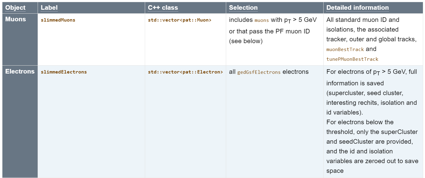
The objects in the MiniAOD format are C++ classes in CMSSW, the CMS Software package, and the table gives the class name corresponding to the physics object. We can find the exact class description in the CMSSW reference manual. See, for example
- Muons:
pat::Muon - Electrons:
pat::Electron.
These are C++ classes that can inherit information from parent classes, or contain objects of some complex types. Therefore, some of the variables are not explicitly listed as they are available through other objects.
Exercise 1: Find NanoAOD variables in MiniAOD
Compare the physics object information available in NanoAOD and MiniAOD.
Can you find the basic variables such as charge,
eta and pt for electrons?
For NanoAOD, see for example the SingleElectron
dataset. You will find Electron_charge,
Electron_eta and Electron_pt in the
listing.
For MiniAOD, read the general description in the WorkBook
and open the reference page for pat::Electron.
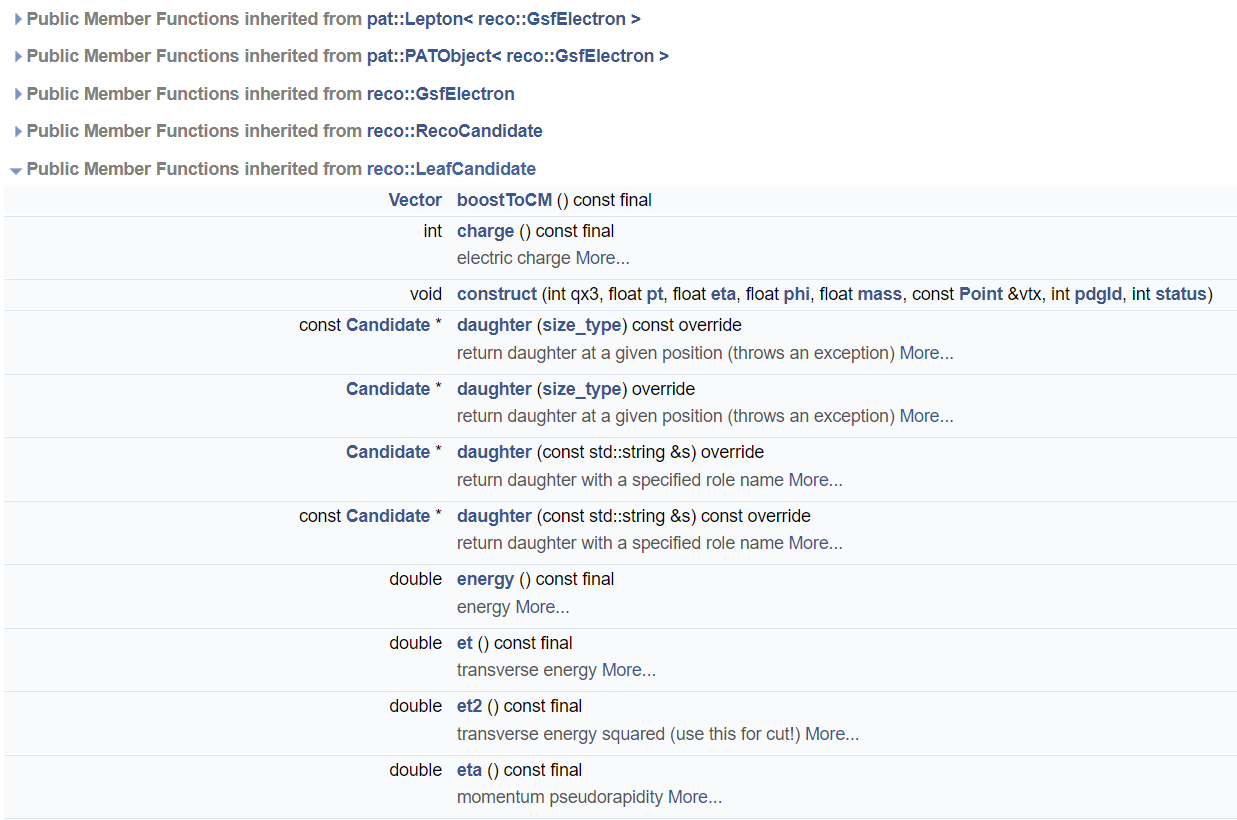
For MiniAOD, we will not find charge, eta
or pt explicitly in the class description as they were
functions inherited from reco::LeafCandidate. This is
transparent in the code when accessing those values, but much less so in
the documentation! You can expand the list of functions inherited for
each parent class in the reference manual page:
Let us now see what information is in MiniAOD but not in NanoAOD. The major difference is that MiniAOD contains most of the constituents of a physics object (such as tracks and/or calorimeter clusters) whereas NanoAOD only contains some information about them.
Exercise 2: Find MiniAOD information that is not in NanoAOD
Compare the physics object information available in NanoAOD and MiniAOD.
Find information about the calorimeter cluster and the track connected to an electron.
In MiniAOD, access to the track information is provided through a
member function gsfTrack.
The full track information is not available in NanoAOD, but it contains, for example, the most pertinent information from its associated track: its impact parameter with respect to the primary interaction vertex. This information is available in NanoAOD variable , read more about it in the pre-learning material.
NanoAOD with Particle Flow candidates
Many CMS open data users have relied on the Particle
Flow information, available in the AOD and MiniAOD formats but not
in the NanoAOD format. See the class description: pat::PackedCandidate.
For the 2016 collision data, a selection of datasets has been processed in NanoAOD format enhanced with Particle Flow information. These datasets can be used in the same way as the usual NanoAOD datasets, they just contain more information.
Exercise 3: Find the datasets in NanoAOD format enhanced with Particle Flow information
Use the CERN Open Data portal search facets to find these derived datasets.
Hint: look at the options under “File type”.
Compare the variable list with the standard NanoAOD.
You can find them by searching
nanoaod-pf.
Select one, find the variable list. Note the section called PFCands
with information about Particle Flow candidates.
An example workflow is provided (and linked to the dataset record) to show how other datasets can be processed into this enhanced format. In principle, it can be used as such, just changing the MiniAOD input dataset name, executing the code in the CMSSW Docker container.
Processing MiniAOD to custom NanoAOD takes time and resources
Processing an entire MiniAOD to custom NanoAOD (i.e. selecting your own objects of interest in addition to those already available in NanoAOD) takes computing resources well beyond a single computer.
Using MiniAOD
If you need the maximum coverage of CMS physics objects, know that CMS provides all that is needed to use data in the MiniAOD format.
You would first find the CMSSW container image with a version corresponding to the data release, and you would start a container in a similar manner as you did for the Python tools and Root containers that we will use in the workshop.
We will not work through it now but if you started the CMSSW container, you would get a container prompt with the CMSSW working area:
BASH
CMSSW should now be available.
This is a standalone image for CMSSW_10_6_30 slc7_amd64_gcc700.
(/code/CMSSW_10_6_30/src)
In this environment, you would be able to follow the instructions in
Getting
started with miniAOD, and, for example, inspect the event content
with CMSSW tools, e.g. with edmDumpEventContent.
Find a file name in the file listing of the SingleElectron MiniAOD record and dump its contents with
BASH
(/code/CMSSW_10_6_30/src) edmDumpEventContent root://eospublic.cern.ch//eos/opendata/cms/Run2016G/SingleElectron/MINIAOD/UL2016_MiniAODv2-v2/120000/0014ADC0-08B8-1347-B496-CDB3A3A32317.root
Type                                  Module                      Label             Process
----------------------------------------------------------------------------------------------
edm::TriggerResults                   "TriggerResults"            ""                "HLT"
BXVector<GlobalAlgBlk>                "gtStage2Digis"             ""                "RECO"
BXVector<GlobalExtBlk>                "gtStage2Digis"             ""                "RECO"
BXVector<l1t::EGamma>                 "caloStage2Digis"           "EGamma"          "RECO"
BXVector<l1t::EtSum>                  "caloStage2Digis"           "EtSum"           "RECO"
BXVector<l1t::Jet>                    "caloStage2Digis"           "Jet"             "RECO"
BXVector<l1t::Muon>                   "gmtStage2Digis"            "Muon"            "RECO"
BXVector<l1t::Tau>                    "caloStage2Digis"           "Tau"             "RECO"
HcalNoiseSummary                      "hcalnoise"                 ""                "RECO"
L1GlobalTriggerReadoutRecord          "gtDigis"                   ""                "RECO"
double                                "fixedGridRhoAll"           ""                "RECO"
double                                "fixedGridRhoFastjetAll"    ""                "RECO"
double                                "fixedGridRhoFastjetAllCalo"   ""                "RECO"
double                                "fixedGridRhoFastjetAllTmp"   ""                "RECO"
double                                "fixedGridRhoFastjetCentral"   ""                "RECO"
double                                "fixedGridRhoFastjetCentralCalo"   ""                "RECO"
double                                "fixedGridRhoFastjetCentralChargedPileUp"   ""                "RECO"
double                                "fixedGridRhoFastjetCentralNeutral"   ""                "RECO"
edm::TriggerResults                   "TriggerResults"            ""                "RECO"
reco::BeamHaloSummary                 "BeamHaloSummary"           ""                "RECO"
reco::BeamSpot                        "offlineBeamSpot"           ""                "RECO"
reco::CSCHaloData                     "CSCHaloData"               ""                "RECO"
vector<CTPPSLocalTrackLite>           "ctppsLocalTrackLiteProducer"   ""                "RECO"
vector<LumiScalers>                   "scalersRawToDigi"          ""                "RECO"
vector<l1extra::L1EmParticle>         "l1extraParticles"          "Isolated"        "RECO"
vector<l1extra::L1EmParticle>         "l1extraParticles"          "NonIsolated"     "RECO"
vector<l1extra::L1EtMissParticle>     "l1extraParticles"          "MET"             "RECO"
vector<l1extra::L1EtMissParticle>     "l1extraParticles"          "MHT"             "RECO"
vector<l1extra::L1HFRings>            "l1extraParticles"          ""                "RECO"
vector<l1extra::L1JetParticle>        "l1extraParticles"          "Central"         "RECO"
vector<l1extra::L1JetParticle>        "l1extraParticles"          "Forward"         "RECO"
vector<l1extra::L1JetParticle>        "l1extraParticles"          "IsoTau"          "RECO"
vector<l1extra::L1JetParticle>        "l1extraParticles"          "Tau"             "RECO"
vector<l1extra::L1MuonParticle>       "l1extraParticles"          ""                "RECO"
vector<reco::Conversion>              "gsfTracksOpenConversions"   "gsfTracksOpenConversions"   "RECO"
vector<reco::ForwardProton>           "ctppsProtons"              "multiRP"         "RECO"
vector<reco::ForwardProton>           "ctppsProtons"              "singleRP"        "RECO"
vector<reco::Track>                   "displacedStandAloneMuons"   ""                "RECO"
BXVector<GlobalExtBlk>                "simGtExtUnprefireable"     ""                "PAT"
double                                "prefiringweight"           "nonPrefiringProb"   "PAT"
double                                "prefiringweight"           "nonPrefiringProbDown"   "PAT"
double                                "prefiringweight"           "nonPrefiringProbUp"   "PAT"
edm::Association<vector<reco::DeDxHitInfo> >    "isolatedTracks"            ""                "PAT"
edm::OwnVector<TrackingRecHit,edm::ClonePolicy<TrackingRecHit> >    "slimmedMuonTrackExtras"    ""                "PAT"
edm::OwnVector<reco::BaseTagInfo,edm::ClonePolicy<reco::BaseTagInfo> >    "slimmedJetsPuppi"          "tagInfos"        "PAT"
edm::RangeMap<CSCDetId,edm::OwnVector<CSCSegment,edm::ClonePolicy<CSCSegment> >,edm::ClonePolicy<CSCSegment> >    "slimmedMuons"              ""                "PAT"
edm::RangeMap<DTChamberId,edm::OwnVector<DTRecSegment4D,edm::ClonePolicy<DTRecSegment4D> >,edm::ClonePolicy<DTRecSegment4D> >    "slimmedMuons"              ""
"PAT"
edm::SortedCollection<EcalRecHit,edm::StrictWeakOrdering<EcalRecHit> >    "reducedEgamma"             "reducedEBRecHits"   "PAT"
edm::SortedCollection<EcalRecHit,edm::StrictWeakOrdering<EcalRecHit> >    "reducedEgamma"             "reducedEERecHits"   "PAT"
edm::SortedCollection<EcalRecHit,edm::StrictWeakOrdering<EcalRecHit> >    "reducedEgamma"             "reducedESRecHits"   "PAT"
edm::SortedCollection<HBHERecHit,edm::StrictWeakOrdering<HBHERecHit> >    "reducedEgamma"             "reducedHBHEHits"   "PAT"
edm::SortedCollection<HBHERecHit,edm::StrictWeakOrdering<HBHERecHit> >    "slimmedHcalRecHits"        "reducedHcalRecHits"   "PAT"
edm::SortedCollection<HFRecHit,edm::StrictWeakOrdering<HFRecHit> >    "slimmedHcalRecHits"        "reducedHcalRecHits"   "PAT"
edm::SortedCollection<HORecHit,edm::StrictWeakOrdering<HORecHit> >    "slimmedHcalRecHits"        "reducedHcalRecHits"   "PAT"
edm::TriggerResults                   "TriggerResults"            ""                "PAT"
edm::ValueMap<float>                  "offlineSlimmedPrimaryVertices"   ""                "PAT"
pat::PackedTriggerPrescales           "patTrigger"                ""                "PAT"
pat::PackedTriggerPrescales           "patTrigger"                "l1max"           "PAT"
pat::PackedTriggerPrescales           "patTrigger"                "l1min"           "PAT"
vector<CTPPSLocalTrackLite>           "ctppsLocalTrackLiteProducer"   ""                "PAT"
vector<pat::CompositeCandidate>       "oniaPhotonCandidates"      "conversions"     "PAT"
vector<pat::Electron>                 "slimmedElectrons"          ""                "PAT"
vector<pat::Electron>                 "slimmedLowPtElectrons"     ""                "PAT"
vector<pat::IsolatedTrack>            "isolatedTracks"            ""                "PAT"
vector<pat::Jet>                      "slimmedJets"               ""                "PAT"
vector<pat::Jet>                      "slimmedJetsAK8"            ""                "PAT"
vector<pat::Jet>                      "slimmedJetsPuppi"          ""                "PAT"
vector<pat::Jet>                      "slimmedJetsAK8PFPuppiSoftDropPacked"   "SubJets"         "PAT"
vector<pat::MET>                      "slimmedMETs"               ""                "PAT"
vector<pat::MET>                      "slimmedMETsNoHF"           ""                "PAT"
vector<pat::MET>                      "slimmedMETsPuppi"          ""                "PAT"
vector<pat::Muon>                     "slimmedMuons"              ""                "PAT"
vector<pat::PackedCandidate>          "lostTracks"                ""                "PAT"
vector<pat::PackedCandidate>          "packedPFCandidates"        ""                "PAT"
vector<pat::PackedCandidate>          "lostTracks"                "eleTracks"       "PAT"
vector<pat::Photon>                   "slimmedOOTPhotons"         ""                "PAT"
vector<pat::Photon>                   "slimmedPhotons"            ""                "PAT"
vector<pat::Tau>                      "slimmedTaus"               ""                "PAT"
vector<pat::Tau>                      "slimmedTausBoosted"        ""                "PAT"
vector<pat::TriggerObjectStandAlone>    "slimmedPatTrigger"         ""                "PAT"
vector<reco::CaloCluster>             "reducedEgamma"             "reducedEBEEClusters"   "PAT"
vector<reco::CaloCluster>             "reducedEgamma"             "reducedESClusters"   "PAT"
vector<reco::CaloCluster>             "reducedEgamma"             "reducedOOTEBEEClusters"   "PAT"
vector<reco::CaloCluster>             "reducedEgamma"             "reducedOOTESClusters"   "PAT"
vector<reco::CaloJet>                 "slimmedCaloJets"           ""                "PAT"
vector<reco::Conversion>              "reducedEgamma"             "reducedConversions"   "PAT"
vector<reco::Conversion>              "reducedEgamma"             "reducedSingleLegConversions"   "PAT"
vector<reco::DeDxHitInfo>             "isolatedTracks"            ""                "PAT"
vector<reco::ForwardProton>           "ctppsProtons"              "multiRP"         "PAT"
vector<reco::ForwardProton>           "ctppsProtons"              "singleRP"        "PAT"
vector<reco::GsfElectronCore>         "reducedEgamma"             "reducedGedGsfElectronCores"   "PAT"
vector<reco::GsfTrack>                "reducedEgamma"             "reducedGsfTracks"   "PAT"
vector<reco::PhotonCore>              "reducedEgamma"             "reducedGedPhotonCores"   "PAT"
vector<reco::PhotonCore>              "reducedEgamma"             "reducedOOTPhotonCores"   "PAT"
vector<reco::SuperCluster>            "reducedEgamma"             "reducedOOTSuperClusters"   "PAT"
vector<reco::SuperCluster>            "reducedEgamma"             "reducedSuperClusters"   "PAT"
vector<reco::TrackExtra>              "slimmedMuonTrackExtras"    ""                "PAT"
vector<reco::Vertex>                  "offlineSlimmedPrimaryVertices"   ""                "PAT"
vector<reco::VertexCompositePtrCandidate>    "slimmedKshortVertices"     ""                "PAT"
vector<reco::VertexCompositePtrCandidate>    "slimmedLambdaVertices"     ""                "PAT"
vector<reco::VertexCompositePtrCandidate>    "slimmedSecondaryVertices"   ""                "PAT"
vector<string>                        "slimmedPatTrigger"         "filterLabels"    "PAT"
unsigned int                          "bunchSpacingProducer"      ""                "PAT"
You would follow the instructions to build a CMSSW analyzer module of your own to select the events and physics object of interest, compile the code and run the analysis in the container. The CMSSW output files are in the Root format and you could use the Python tools or the Root container to analyze them further.
The previous workshops have extensive learning material for using CMSSW with MiniAOD (or AOD) data formats. Feel free to explore them!
Key Points
- Analyses that require detailed information about physics object constituents may require using MiniAOD instead of NanoAOD
- Selected datasets include Particle Flow candidates in an enriched NanoAOD format are available and their use does not require using CMS-specific software
- CMSSW environment is available as a Docker container and can be used to work with MiniAOD
Content from NanoAOD datasets
Last updated on 2024-07-29 | Edit this page
Estimated time: 30 minutes
Overview
Questions
- How do we find a specific nanoAOD dataset?
- How to we explore the content of our nanoAOD dataset?
Objectives
- Know how to find nanoAOD datasets
- Know how to explore the content of nanoAOD
Find and explore a nanoAOD dataset
Let’s find and explore a particular which we will get even further into later: simulated Z’ events in which the Z’ decays to a top and antitop quark pair.
Callout
A Z’ (“Z-prime”) is a hypothetical heavy gauge boson that could come from extensions of the Standard Model. A review of searches for the Z’ can be found here
Find the dataset
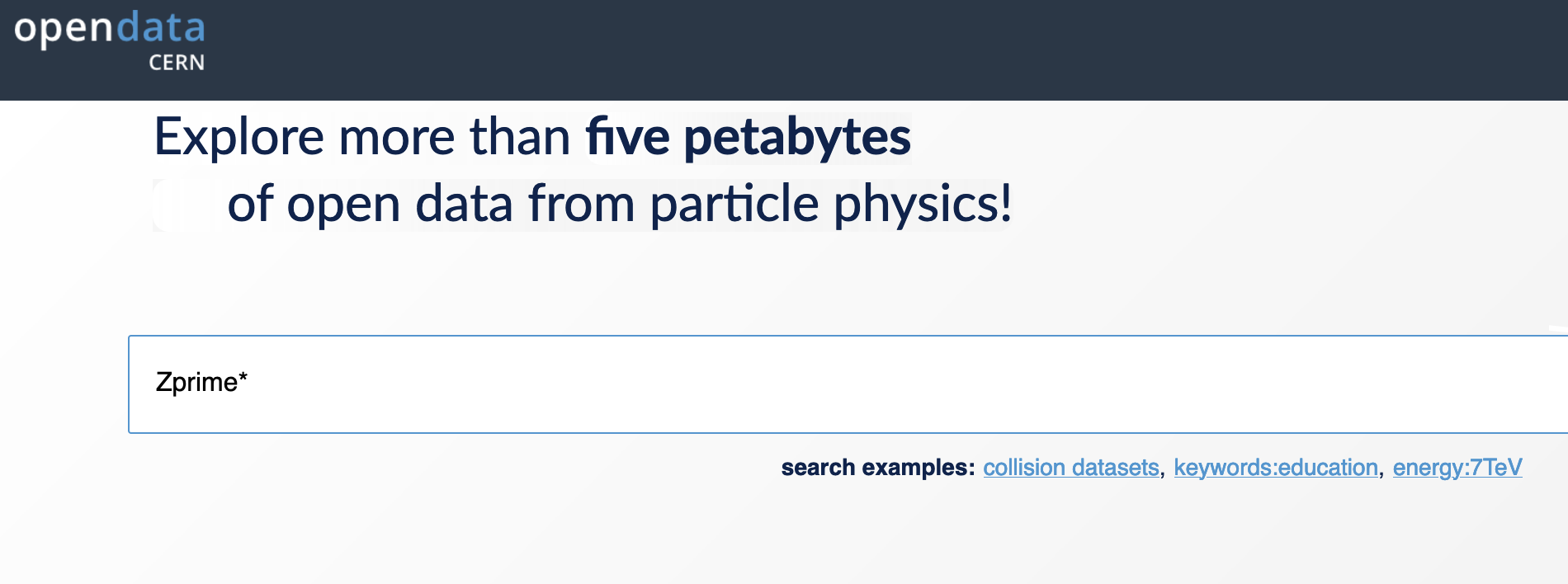
All data can be found via the CERN Open Data Portal. Let’s go to the website and search the simulated Z’ datasets.
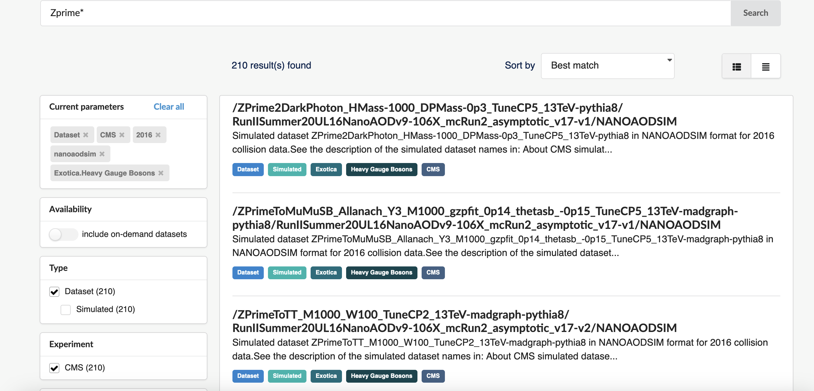
Dataset naming in CMS can seem obscure but let’s do something simple and search for “Zprime*“:
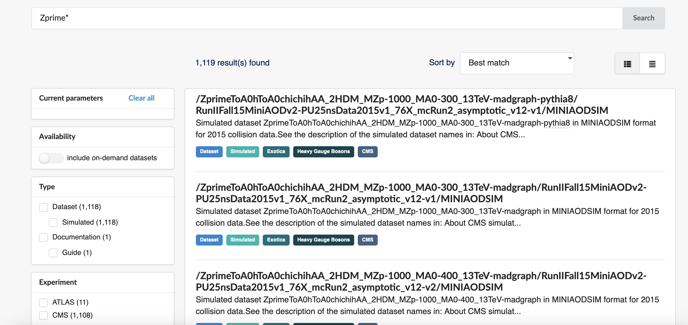
The query results are here and you can see that there are many (over 1000) records returned:
Let’s narrow down the results and select Dataset under Type, CMS under Experiment, 2016 under “Year”, nanoaodsim under File type, and Heavy Gauge Bosons under Category. We’ve now reduced the number of matches from over 1000 down to 210:
We can discern some of the logic behind the simulated dataset naming. “Zprime” is the particle produced and it decays to various products. We want \(Z^{'} \rightarrow t\bar{t}\) which shows up as the third result so let’s narrow the search further and search with “ZprimeToTT*“:
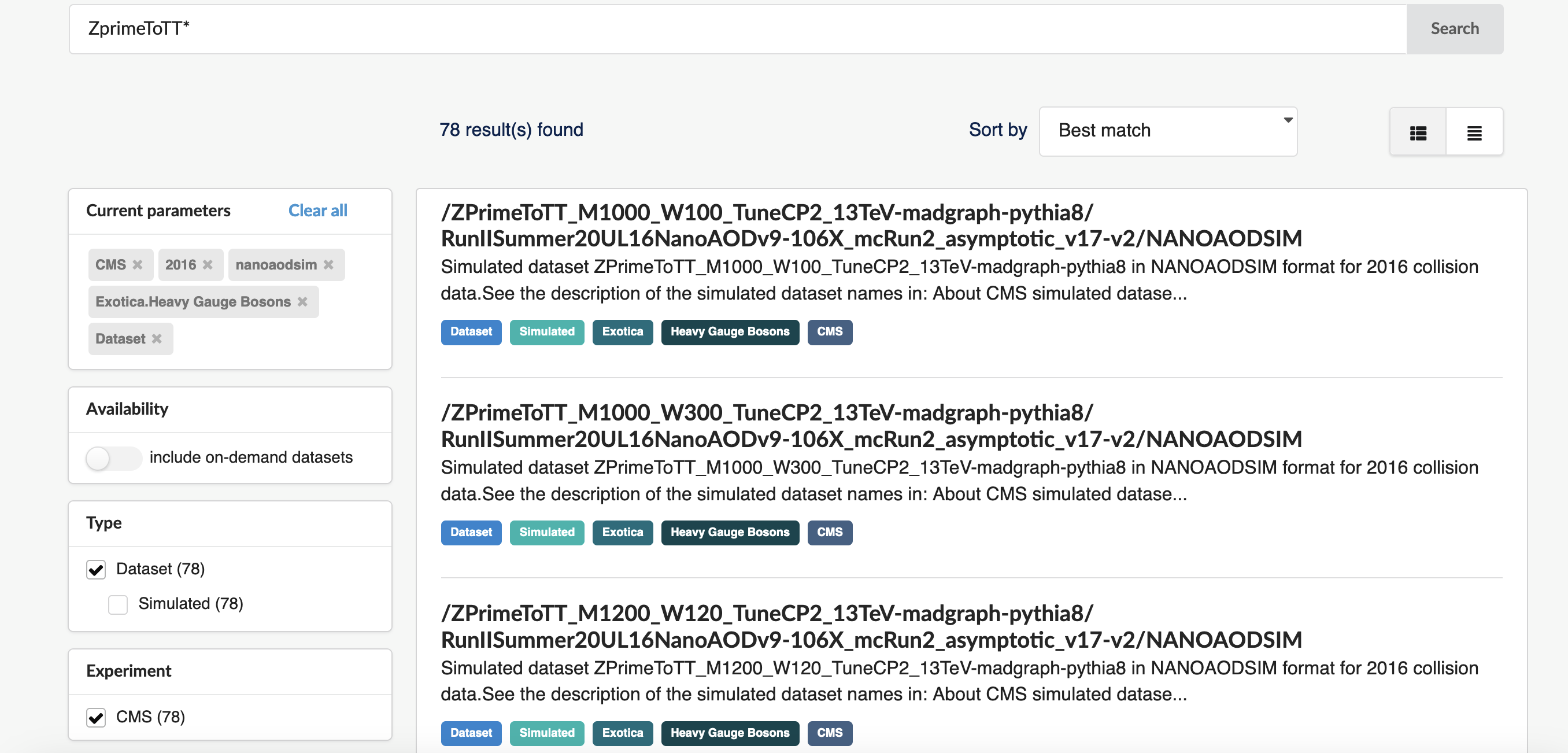
We can also discern that the dataset names also include the mass (in GeV) of the hypothetical Z’ (e.g. “_M2000”).
Why such long dataset names?
CMS open data are the same files that have been used in the data analysis by CMS members. The names come from naming conventions for the production system.
Go back to the pre-exercise for a brief explanation of the simulated dataset names.
Exercise 1: Select a Z’ mass and find the corresponding dataset
Search with “ZprimeToTT_M<mass>” where
<mass> is the value you selected.
Next, let’s use the cernopendata-client command-line
tool to find the datasets and fetch a file.
Exercise 2: Find a file name in the dataset
Go back to the pre-exercise to see how to get the file names with the command-line tool.
Explore a file
We will now have a look at the file contents.
How to know what variables are there?
Remember that each NanoAOD/NanoAODSIM dataset has the variable list linked to the record:
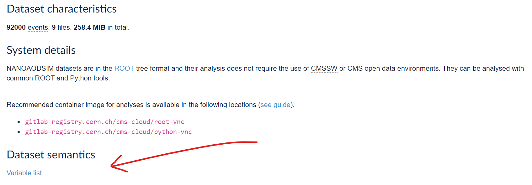
And do not forget that the prelearning lesson on Physics Objects explains them in more detail!
Now let us plot the value of some these variables. Open the
my_python container
You can either write your code in a Python script, or use a jupyter notebook.
If you want to use jupyter notebooks, start jupyter-lab with
Open the link given in the message on your browser. Choose the icon under “Notebook”.
Exercise 3: Explore the file with the Python tools
Open the file and print the variable names.
Make a plot of a variable that is a single number in an event, for example the number of secondary vertices.
Then plot some property of the selected variables, for example a property of the secondary vertices.
Go back to the pre-exercise to see how to open the file using uproot.
If you need exercising, try to do this without looking at the solutions!
First import the Python packages.
Open the file with uproot and inspect the first
layer.
Check what variables are available in Events.
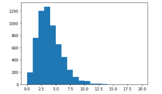
Choose first a variable that is a single number in an event,
typically a number of certain objects in an event. You could take number
of muons, electrons or other particles, but let us take the number of
secondary vertices, nSV. They are points identified as
starting points of a track, different from the collision point, the
primary vertex. It is typically the decay point of some short-lived
particle. Make a histogram.
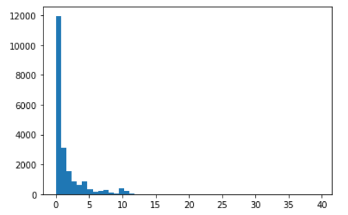
Then, choose a variable of a physics object that can be many in a
single event. You could take the pt values of electrons or muons, or if
we remain with the secondary vertices, take for example
SV_dxy, the 2D decay length in cm.
This is now a jagged array and to plot the values, you will
need to use the flatten() function from
awkward.
But first, inspect the array elements to see the multiple values per event
Print the number or secondary vertices per event (the value we just plotted):
Now, print the 2D decay lengths:
and some single elements of it so that you see that the lenght of corresponds to the number of secondary vertices:
Key Points
- Use search facets and text search with wildcards to narrow your search.
- You can find the variable names with a brief explanation from the record, explained more in detail in the prelearning lesson and print them out directly from the file.
- NanoAOD files can be opened using the
uprootpackage and theawkwardpackaged can be use to handle varying-length arrays.