Electrons & Photons
Last updated on 2024-07-09 | Edit this page
Estimated time: 10 minutes
Overview
Questions
- What are electromagnetic objects
- How are electrons treated in CMS?
- What variables are available in NanoAOD?
Objectives
- Understand what electromagnetic objects are in CMS
- Learn electron member functions for common track-based quantities
- Learn variables for identification and isolation of electrons
- Learn variables for electron detector-related quantities
Motivation
In the middle of the workshop we will be working on the main activity, which is to attempt to replicate a CMS physics analysis in a simplified way using modern analysis tools. The final state that we will be looking at contains electrons, muons and jets. We are using these objects as examples to review the way in which we extract physics objects information.
The analysis requires some special variables, which we will need to identify in our Open Data NanoAOD files.
Electromagnetic objects
We call photons and electrons electromagnetic particles because they leave most of their energy in the electromagnetic calorimeter (ECAL) so they share many common properties and functions
Many of the different hypothetical exotic particles are unstable and can transform, or decay, into electrons, photons, or both. Electrons and photons are also standard tools to measure better and understand the properties of already known particles. For example, one way to find a Higgs Boson is by looking for signs of two photons, or four electrons in the debris of high energy collisions. Because electrons and photons are crucial in so many different scenarios, the physicists in the CMS collaboration make sure to do their best to reconstruct and identify these objects.
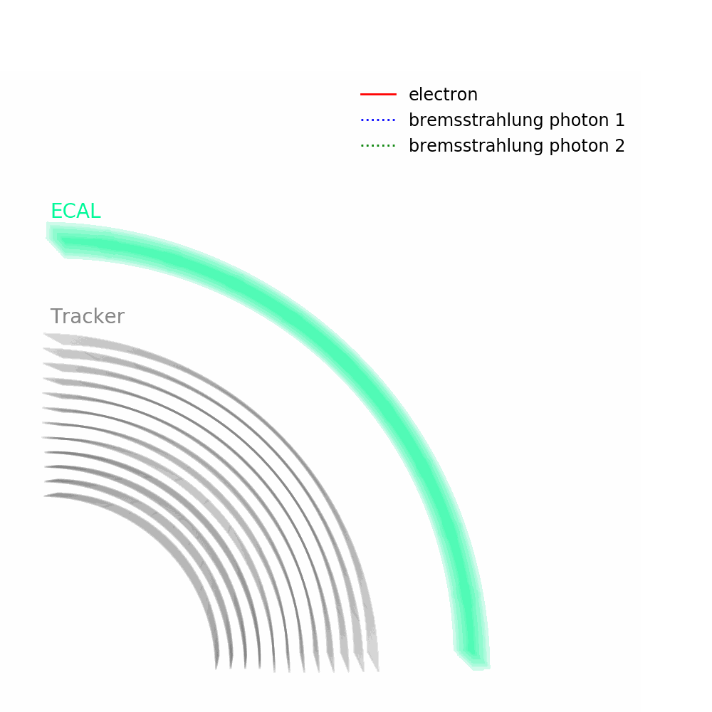
As depicted in the figure above, tracks – from the pixel and silicon tracker systems – as well as ECAL energy deposits are used to identify the passage of electrons in CMS. Being charged, electron trajectories curve inside the CMS magnetic field. Photons are similar objects but with no tracks. Sophisticated algorithms are run in the reconstruction to take into account subtleties related to the identification of an electromagnetic particle. An example is the convoluted showering of sub-photons and sub-electrons that can reach the ECAL due to bremsstrahlung and photon conversions.
We measure momentum and energy but also other properties of these objects that help analysts understand better their quality and origin.
Electron variables in NanoAOD
In the pre-exercises, you learned how to find NanoAOD datasets on the
Open Data Portal. One example is the SingleElectron dataset.
The “Dataset Semantics” section has a link to the variable
list webpage. Each “collection” of objects in the NanoAOD file is
linked by a common naming scheme (ex: Electron_*). The
individual variables are shown in a table that includes the branch name,
the data type, and a brief descriptive comment.
| Object property | Type | Description |
|---|---|---|
| Electron_charge | Int_t | electric charge |
| Electron_cleanmask | UChar_t | simple cleaning mask with priority to leptons |
| Electron_convVeto | Bool_t | pass conversion veto |
| Electron_cutBased | Int_t | cut-based ID Fall17 V2 (0:fail, 1:veto, 2:loose, 3:medium, 4:tight) |
| Electron_cutBased_HEEP | Bool_t | cut-based HEEP ID |
| Electron_dEscaleDown | Float_t | ecal energy scale shifted 1 sigma down (adding gain/stat/syst in quadrature) |
| Electron_dEscaleUp | Float_t | ecal energy scale shifted 1 sigma up(adding gain/stat/syst in quadrature) |
| Electron_dEsigmaDown | Float_t | ecal energy smearing value shifted 1 sigma up |
| Electron_dEsigmaUp | Float_t | ecal energy smearing value shifted 1 sigma up |
| Electron_deltaEtaSC | Float_t | delta eta (SC,ele) with sign |
| Electron_dr03EcalRecHitSumEt | Float_t | Non-PF Ecal isolation within a delta R cone of 0.3 with electron pt > 35 GeV |
| Electron_dr03HcalDepth1TowerSumEt | Float_t | Non-PF Hcal isolation within a delta R cone of 0.3 with electron pt > 35 GeV |
| Electron_dr03TkSumPt | Float_t | Non-PF track isolation within a delta R cone of 0.3 with electron pt > 35 GeV |
| Electron_dr03TkSumPtHEEP | Float_t | Non-PF track isolation within a delta R cone of 0.3 with electron pt > 35 GeV used in HEEP ID |
| Electron_dxy | Float_t | dxy (with sign) wrt first PV, in cm |
| Electron_dxyErr | Float_t | dxy uncertainty, in cm |
| Electron_dz | Float_t | dz (with sign) wrt first PV, in cm |
| Electron_dzErr | Float_t | dz uncertainty, in cm |
| Electron_eCorr | Float_t | ratio of the calibrated energy/miniaod energy |
| Electron_eInvMinusPInv | Float_t | 1/E_SC - 1/p_trk |
| Electron_energyErr | Float_t | energy error of the cluster-track combination |
| Electron_eta | Float_t | eta |
| Electron_hoe | Float_t | H over E |
| Electron_ip3d | Float_t | 3D impact parameter wrt first PV, in cm |
| Electron_isPFcand | Bool_t | electron is PF candidate |
| Electron_jetIdx | Int_t | (index to Jet) index of the associated jet (-1 if none) |
| Electron_jetNDauCharged | UChar_t | number of charged daughters of the closest jet |
| Electron_jetPtRelv2 | Float_t | Relative momentum of the lepton with respect to the closest jet after subtracting the lepton |
| Electron_jetRelIso | Float_t | Relative isolation in matched jet (1/ptRatio-1, pfRelIso04_all if no matched jet) |
| Electron_lostHits | UChar_t | number of missing inner hits |
| Electron_mass | Float_t | mass |
| Electron_miniPFRelIso_all | Float_t | mini PF relative isolation, total (with scaled rho*EA PU corrections) |
| Electron_miniPFRelIso_chg | Float_t | mini PF relative isolation, charged component |
| Electron_mvaFall17V2Iso | Float_t | MVA Iso ID V2 score |
| Electron_mvaFall17V2Iso_WP80 | Bool_t | MVA Iso ID V2 WP80 |
| Electron_mvaFall17V2Iso_WP90 | Bool_t | MVA Iso ID V2 WP90 |
| Electron_mvaFall17V2Iso_WPL | Bool_t | MVA Iso ID V2 loose WP |
| Electron_mvaFall17V2noIso | Float_t | MVA noIso ID V2 score |
| Electron_mvaFall17V2noIso_WP80 | Bool_t | MVA noIso ID V2 WP80 |
| Electron_mvaFall17V2noIso_WP90 | Bool_t | MVA noIso ID V2 WP90 |
| Electron_mvaFall17V2noIso_WPL | Bool_t | MVA noIso ID V2 loose WP |
| Electron_mvaTTH | Float_t | TTH MVA lepton ID score |
| Electron_pdgId | Int_t | PDG code assigned by the event reconstruction (not by MC truth) |
| Electron_pfRelIso03_all | Float_t | PF relative isolation dR=0.3, total (with rho*EA PU corrections) |
| Electron_pfRelIso03_chg | Float_t | PF relative isolation dR=0.3, charged component |
| Electron_phi | Float_t | phi |
| Electron_photonIdx | Int_t | (index to Photon) index of the associated photon (-1 if none) |
| Electron_pt | Float_t | p_{T} |
| Electron_r9 | Float_t | R9 of the supercluster, calculated with full 5x5 region |
| Electron_scEtOverPt | Float_t | (supercluster transverse energy)/pt-1 |
| Electron_seedGain | UChar_t | Gain of the seed crystal |
| Electron_sieie | Float_t | sigma_IetaIeta of the supercluster, calculated with full 5x5 region |
| Electron_sip3d | Float_t | 3D impact parameter significance wrt first PV, in cm |
| Electron_tightCharge | Int_t | Tight charge criteria (0:none, 1:isGsfScPixChargeConsistent, 2:isGsfCtfScPixChargeConsistent) |
| Electron_vidNestedWPBitmap | Int_t | VID compressed bitmap (MinPtCut,GsfEleSCEtaMultiRangeCut,GsfEleDEtaInSeedCut,GsfEleDPhiInCut,GsfEleFull5x5SigmaIEtaIEtaCut,GsfEleHadronicOverEMEnergyScaledCut,GsfEleEInverseMinusPInverseCut,GsfEleRelPFIsoScaledCut,GsfEleConversionVetoCut,GsfEleMissingHitsCut), 3 bits per cut |
| Electron_vidNestedWPBitmapHEEP | Int_t | VID compressed bitmap (MinPtCut,GsfEleSCEtaMultiRangeCut,GsfEleDEtaInSeedCut,GsfEleDPhiInCut,GsfEleFull5x5SigmaIEtaIEtaWithSatCut,GsfEleFull5x5E2x5OverE5x5WithSatCut,GsfEleHadronicOverEMLinearCut,GsfEleTrkPtIsoCut,GsfEleEmHadD1IsoRhoCut,GsfEleDxyCut,GsfEleMissingHitsCut,GsfEleEcalDrivenCut), 1 bits per cut |
| nElectron | UInt_t | slimmedElectrons after basic selection (pt > 5 ) |
Electron 4-vector and track information
All CMS physics objects contain basic 4-vector information: transverse momentum, pseudorapidity, azimuthal angle, and mass or energy:
| Object property | Type | Description |
|---|---|---|
| Electron_eta | Float_t | eta |
| Electron_mass | Float_t | mass |
| Electron_phi | Float_t | phi |
| Electron_pt | Float_t | p_{T} |
Most charged physics objects are also connected to tracks from the
CMS tracking detectors, and therefore the electric charge can be
identified from the track curvature. Electron charge can be computed
from 3 unique algorithms, so a tightCharge variable exists
to show when multiple of the charge determinations agree. Information
from tracks provides other kinematic quantities that are common to
multiple types of objects. Often, the most pertinent information about
an object to access from its associated track is its impact
parameter with respect to the primary interaction vertex. We
can access the impact parameters in the xy-plane (dxy or
d0) and along the beam axis (dz), as well as
their respective uncertainties. There is also a 3D impact parameter
significance that is very useful for identifying leptons that emerged
from a heavy flavor hadron decay.
| Object property | Type | Description |
|---|---|---|
| Electron_charge | Int_t | electric charge |
| Electron_dxy | Float_t | dxy (with sign) wrt first PV, in cm |
| Electron_dxyErr | Float_t | dxy uncertainty, in cm |
| Electron_dz | Float_t | dz (with sign) wrt first PV, in cm |
| Electron_dzErr | Float_t | dz uncertainty, in cm |
| Electron_sip3d | Float_t | 3D impact parameter significance wrt first PV, in cm |
| Electron_tightCharge | Int_t | Tight charge criteria (0:none, 1:isGsfScPixChargeConsistent, 2:isGsfCtfScPixChargeConsistent) |
Track-based info for photons
Note: in the case of Photons, since they are neutral objects, they do
not have a direct track link (though displaced track segments may appear
from electrons or positrons produced by the photon as it transits the
detector material). While the charge variable exists for
all objects, it is not used in photon analyses.
Detector information for identification
The most signicant difference between a list of certain particles from a Monte Carlo generator and a list of the corresponding physics objects from CMS is likely the inherent uncertainty in the reconstruction. Selection of “a muon” or “an electron” for analysis requires algorithms designed to separate “real” objects from “fakes”. These are called identification algorithms.
Other algorithms are designed to measure the amount of energy deposited near the object, to determine if it was likely produced near the primary interaction (typically little nearby energy), or from the decay of a longer-lived particle (typically a lot of nearby energy). These are called isolation algorithms. Many types of isolation algorithms exist to deal with unique physics cases!
Both types of algorithms function using working points that are described on a spectrum from “loose” to “tight”. Working points that are “looser” tend to have a high efficiency for accepting real objects, but perhaps a poor rejection rate for “fake” objects. Working points that are “tighter” tend to have lower efficiencies for accepting real objects, but much better rejection rates for “fake” objects. The choice of working point is highly analysis dependent! Some analyses value efficiency over background rejection, and some analyses are the opposite.
The standard identification and isolation algorithm results can be accessed from the physics object classes.
Multivariate Electron Identification (MVA)
In the Multi-variate Analysis (MVA) approach, one forms a single discriminator variable that is computed based on multiple parameters of the electron object and provides the best separation between the signal and backgrounds by means of multivariate analysis methods and statistical learning tools. One can then cut on discriminator value or use the distribution of the values for a shape based statistical analysis.
There are two basic types of MVAs that are were trained by CMS for 2016 electrons:
- MVA with isolation: the MVA includes standard particle-flow isolation as one of the variables used for training. This MVA is well suited for analyses considering typical prompt electrons that are likely to be isolated from jets or other objects.
- MVA without isolation: no isolation variables are included for training. This MVA is better suited for analyses in which the electrons might be poorly isolated from jets or other objects.
Both MVAs were assigned working points with 80% efficiency (WP80), 90% efficiency (WP90), and a very high efficiency (“loose”)
| Object property | Type | Description |
|---|---|---|
| Electron_mvaFall17V2Iso | Float_t | MVA Iso ID V2 score |
| Electron_mvaFall17V2Iso_WP80 | Bool_t | MVA Iso ID V2 WP80 |
| Electron_mvaFall17V2Iso_WP90 | Bool_t | MVA Iso ID V2 WP90 |
| Electron_mvaFall17V2Iso_WPL | Bool_t | MVA Iso ID V2 loose WP |
| Electron_mvaFall17V2noIso | Float_t | MVA noIso ID V2 score |
| Electron_mvaFall17V2noIso_WP80 | Bool_t | MVA noIso ID V2 WP80 |
| Electron_mvaFall17V2noIso_WP90 | Bool_t | MVA noIso ID V2 WP90 |
| Electron_mvaFall17V2noIso_WPL | Bool_t | MVA noIso ID V2 loose WP |
Cut Based Electron ID
Electron identification can also be evaluated without MVAs, using a set of “cut-based” identification criteria:
| Object property | Type | Description |
|---|---|---|
| Electron_cutBased | Int_t | cut-based ID Fall17 V2 (0:fail, 1:veto, 2:loose, 3:medium, 4:tight) |
| Electron_cutBased_HEEP | Bool_t | cut-based HEEP ID |
Four standard working points are provided * Veto (average efficiency ~95%). Use this working point for third lepton veto or counting. * Loose (average efficiency ~90%). Use this working point when backgrounds are rather low. * Medium (average efficiency ~80%). This is a good starting point for generic measurements involving W or Z bosons. * Tight (average efficiency ~70%). Use this working point for measurements where backgrounds are a serious problem.
All of the cut-based working points include particle-flow isolation
requirements. The HEEP identifier is specifically intended
to improve efficiency for high-energy electrons with more than 100-200
GeV of transverse momentum.
Electron isolation
Isolation is computed in similar ways for all physics objects: search for particles in a cone around the object of interest and sum up their energies, subtracting off the energy deposited by pileup particles. This sum divided by the object of interest’s transverse momentum is called relative isolation and is the most common way to determine whether an object was produced “promptly” in or following the proton-proton collision (ex: electrons from a Z boson decay, or photons from a Higgs boson decay). Relative isolation values will tend to be large for particles that emerged from weak decays of hadrons within jets, or other similar “nonprompt” processes.
While many of the electron identification algorithms include isolation, the isolation values are also available:
| Object property | Type | Description |
|---|---|---|
| Electron_dr03EcalRecHitSumEt | Float_t | Non-PF Ecal isolation within a delta R cone of 0.3 with electron pt > 35 GeV |
| Electron_dr03HcalDepth1TowerSumEt | Float_t | Non-PF Hcal isolation within a delta R cone of 0.3 with electron pt > 35 GeV |
| Electron_dr03TkSumPt | Float_t | Non-PF track isolation within a delta R cone of 0.3 with electron pt > 35 GeV |
| Electron_dr03TkSumPtHEEP | Float_t | Non-PF track isolation within a delta R cone of 0.3 with electron pt > 35 GeV used in HEEP ID |
| Electron_pfRelIso03_all | Float_t | PF relative isolation dR=0.3, total (with rho*EA PU corrections) |
| Electron_pfRelIso03_chg | Float_t | PF relative isolation dR=0.3, charged component |
Electron cross-reference indices
Electrons can be associated with both jets and photons based on the particle-flow algorithm. Since the jet and photon collections have independent array structures, the indices of the matched jet or photon is provided in the electron collection:
| Object property | Type | Description |
|---|---|---|
| Electron_jetIdx | Int_t | (index to Jet) index of the associated jet (-1 if none) |
| Electron_photonIdx | Int_t | (index to Photon) index of the associated photon (-1 if none) |
Photons
Since photons are also primarily reconstructed as electromagnetic calorimeter showers, the vast majority of their reconstruction methods are common with electrons. Photons also have 4-vector, identification, and isolation information available in NanoAOD
| Object property | Type | Description |
|---|---|---|
| Photon_charge | Int_t | electric charge |
| Photon_cleanmask | UChar_t | simple cleaning mask with priority to leptons |
| Photon_cutBased | Int_t | cut-based ID bitmap, Fall17V2, (0:fail, 1:loose, 2:medium, 3:tight) |
| Photon_cutBased_Fall17V1Bitmap | Int_t | cut-based ID bitmap, Fall17V1, 2^(0:loose, 1:medium, 2:tight). |
| Photon_dEscaleDown | Float_t | ecal energy scale shifted 1 sigma down (adding gain/stat/syst in quadrature) |
| Photon_dEscaleUp | Float_t | ecal energy scale shifted 1 sigma up (adding gain/stat/syst in quadrature) |
| Photon_dEsigmaDown | Float_t | ecal energy smearing value shifted 1 sigma up |
| Photon_dEsigmaUp | Float_t | ecal energy smearing value shifted 1 sigma up |
| Photon_eCorr | Float_t | ratio of the calibrated energy/miniaod energy |
| Photon_electronIdx | Int_t (index to Electron) | index of the associated electron (-1 if none) |
| Photon_electronVeto | Bool_t | pass electron veto |
| Photon_energyErr | Float_t | energy error of the cluster from regression |
| Photon_eta | Float_t | eta |
| Photon_hoe | Float_t | H over E |
| Photon_isScEtaEB | Bool_t | is supercluster eta within barrel acceptance |
| Photon_isScEtaEE | Bool_t | is supercluster eta within endcap acceptance |
| Photon_jetIdx | Int_t | (index to Jet) index of the associated jet (-1 if none) |
| Photon_mass | Float_t | mass |
| Photon_mvaID | Float_t | MVA ID score, Fall17V2 |
| Photon_mvaID_Fall17V1p1 | Float_t | MVA ID score, Fall17V1p1 |
| Photon_mvaID_WP80 | Bool_t | MVA ID WP80, Fall17V2 |
| Photon_mvaID_WP90 | Bool_t | MVA ID WP90, Fall17V2 |
| Photon_pdgId | Int_t | PDG code assigned by the event reconstruction (not by MC truth) |
| Photon_pfRelIso03_all | Float_t | PF relative isolation dR=0.3, total (with rho*EA PU corrections) |
| Photon_pfRelIso03_chg | Float_t | PF relative isolation dR=0.3, charged component (with rho*EA PU corrections) |
| Photon_phi | Float_t | phi |
| Photon_pixelSeed | Bool_t | has pixel seed |
| Photon_pt | Float_t | p_{T} |
| Photon_r9 | Float_t | R9 of the supercluster, calculated with full 5x5 region |
| Photon_seedGain | UChar_t | Gain of the seed crystal |
| Photon_sieie | Float_t | sigma_IetaIeta of the supercluster, calculated with full 5x5 region |
| Photon_vidNestedWPBitmap | Int_t | Fall17V2 VID compressed bitmap (MinPtCut,PhoSCEtaMultiRangeCut,PhoSingleTowerHadOverEmCut,PhoFull5x5SigmaIEtaIEtaCut,PhoGenericRhoPtScaledCut,PhoGenericRhoPtScaledCut,PhoGenericRhoPtScaledCut), 2 bits per cut |
| nPhoton | UInt_t | slimmedPhotons after basic selection (pt > 5 ) |
Key Points
- Quantities such as impact parameters and charge have common member functions.
- Physics objects in CMS are reconstructed from detector signals and are never 100% certain!
- Identification and isolation algorithms are important for reducing fake objects.