Jet flavor tagging
Last updated on 2024-07-09 | Edit this page
Estimated time: 20 minutes
Overview
Questions
- How are b hadrons identified in CMS?
- How are the parent particles of large-radius jets identified in CMS?
Objectives
- Understand the basics of heavy flavor tagging
- Learn to access tagging information in NanoAOD files
Jet reconstruction and identification is an important part of the analyses at the LHC. A jet may contain the hadronization products of any quark or gluon, or possibly the decay products of more massive particles such as W or Higgs bosons. Several “b tagging” algorithms exist to identify jets from the hadronization of b quarks, which have unique properties that distinguish them from light quark or gluon jets.
B Tagging Algorithms
Tagging algorithms first connect the jets with good quality tracks that are either associated with one of the jet’s particle flow candidates or within a nearby cone. Both tracks and “secondary vertices” (track vertices from the decays of b hadrons) can be used in track-based, vertex-based, or “combined” tagging algorithms. The specific details depend upon the algorithm use. However, they all exploit properties of b hadrons such as:
- long lifetime,
- large mass,
- high track multiplicity,
- large semileptonic branching fraction,
- hard fragmentation fuction.
In CMS, several b tagging algorithms have existed over time:
- Track Counting: identifies a b jet if it contains at least N tracks with significantly non-zero impact parameters.
- Jet Probability: combines information from all selected tracks in the jet and uses probability density functions to assign a probability to each track
- Soft Muon and Soft Electron: identifies b jets by searching for a lepton from a semi-leptonic b decay.
- Simple Secondary Vertex: reconstructs the b decay vertex and calculates a discriminator using related kinematic variables.
- Combined Secondary Vertex (CSV): exploits all known kinematic variables of the jets, information about track impact parameter significance and the secondary vertices to distinguish b jets. This tagger became the default CMS algorithm in Run 1 and early Run 2.
- DeepCSV: the CSV algorithm was reimagined as a deep neural network.
- DeepJet: this deep neural network tagger uses a more complex architecture than DeepCSV, and is the most powerful b tagging algorithm for Run 2.
These algorithms produce a single, real number called a b tagging “discriminator” for each jet. The more positive the discriminator value, the more likely it is that this jet contained b hadrons. The DeepCSV and DeepJet algorithms can also identify charm-flavor jets, and DeepJet can even distinguish between light-quark and gluon jets.
| Object property | Type | Description |
|---|---|---|
| Jet_btagCSVV2 | Float_t | pfCombinedInclusiveSecondaryVertexV2 b-tag discriminator (aka CSVV2) |
| Jet_btagDeepB | Float_t | DeepCSV b+bb tag discriminator |
| Jet_btagDeepCvB | Float_t | DeepCSV c vs b+bb discriminator |
| Jet_btagDeepCvL | Float_t | DeepCSV c vs udsg discriminator |
| Jet_btagDeepFlavB | Float_t | DeepJet b+bb+lepb tag discriminator |
| Jet_btagDeepFlavCvB | Float_t | DeepJet c vs b+bb+lepb discriminator |
| Jet_btagDeepFlavCvL | Float_t | DeepJet c vs uds+g discriminator |
| Jet_btagDeepFlavQG | Float_t | DeepJet g vs uds discriminator |
Working points
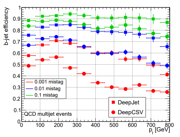
A jet is considered “b tagged” if the discriminator value exceeds some threshold. Different thresholds will have different efficiencies for identifying true b quark jets and for mis-tagging light quark jets. As we saw for muons and other objects, a “loose” working point will allow the highest mis-tagging rate, while a “tight” working point will sacrifice some correct-tag efficiency to reduce mis-tagging. The DeepCSV and DeepJet algorithms are supported by CMS for 2016 Open Data.
The supported working points for DeepCSV and DeepJet for the 2016 Open Data are:
- Loose (10% misidentification rate):
Jet_btagDeepB> 0.1918 ,Jet_btagDeepFlav> 0.0480 - Medium (1% misidentification rate):
Jet_btagDeepB> 0.5847,Jet_btagDeepFlav> 0.2489 - Tight (0.1% misidentification rate):
Jet_btagDeepB> 0.8767,Jet_btagDeepFlav> 0.6377
The figure below shows the relationship between b jet efficiency and working point in DeepCSV and DeepJet:
FatJet tagging algorithms
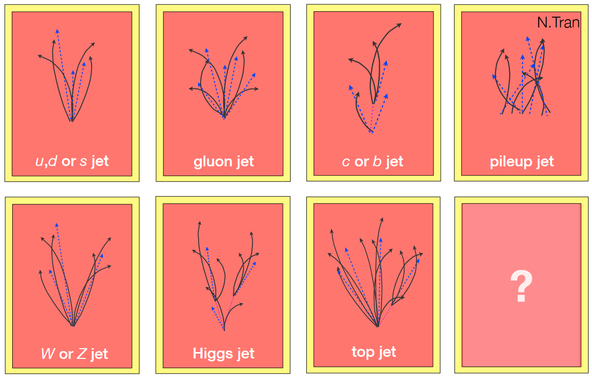
Jets can originate from many different types of particles. The figure below gives an example of how different “parent particles” can influence the internal structure of a jet. Observables related to the mass and internal structure of a jet can help us design algorithms to distinguish between sources. The most common type of algorithm identifies b quark jets from light quark or gluon jets. The POET contains all the tools you need to evaluate the default CMS b tagging discriminants on small-radius jets. See the next episode for more information. In this lesson we will focus on tools to identify hadronic decays of Lorentz-boosed massive SM particles within large-radius jets.
Groomed mass and substructure
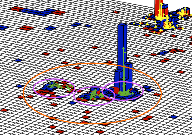
The mass of a jet is evaluated by summing the energy-momentum four-vectors of all the particle flow candidates that make up the jet and computing the mass of the resulting object. This mass calculation is distorted by the low-momentum and wide-angle gluon radiation emerging from the initial hadrons that formed the jet. For example, the masses of light quark or gluon jets are measured to be much larger than the actual masses of these particles – typically 10–50 GeV with a smooth continuum to higher values. Grooming procedures can help reduce the impact of this radiation and bring the jet mass closer to the true values of the parent particles. Grooming algorithms typically cluster the jet’s consitituents into “subjets”, like those represented by the small circles in the figure below. The relationships between different subjets can then be tested to decide which to keep.
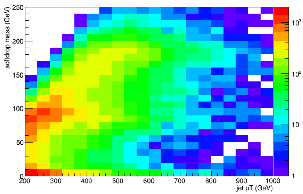
The “softdrop” mass is included in NanoAOD for large-radius jets. In the “softdrop” procedure, jets are recursively de-clustered, and at each step jets that are too soft or at large angles are discarded. The following image shows the relationship between FatJet momentum, mass, and jet radius. As the momentum increases, jets of larger mass become contained within the FatJet. While W bosons can be observed from 200 GeV, top quarks require a higher momentum threshold.
The internal structure of a jet can be probed using many observables: N-subjettiness, energy correlation functions, and others. In CMS, N-subjettiness is the default jet substructure variable for identifying boosted particle decays.
The “tau” variables of N-subjettiness, defined below, are jet shape variables whose value approaches 0 for jets having N or fewer subjets:
\(\tau_{N} = \frac{\sum^{n_{\mathrm{constituents}}}_{i=1} p_{\mathrm{T},i} \min{\Delta R_{1,i}, \Delta R_{2,i}, \ldots, \Delta R_{N,i}}}{\sum^{n_{\mathrm{constituents}}}_{i=1} p_{T,i}R}\)
If the value approaches zero it indicates that the consitituents all lie near one of the previously identified subjet axes. For a top quark jet with 3 subjets, we would expect small tau values for N = 3, 4, 5, 6, etc, but larger values for N = 1 or 2. Ratios of tau values provide the best discrimination for jets with a specific number of subjets. For two-prong jets like W, Z, or H boson decays, we study the ratio tau_2 / tau_1. For three-prong jets we study tau_3 / tau_2.
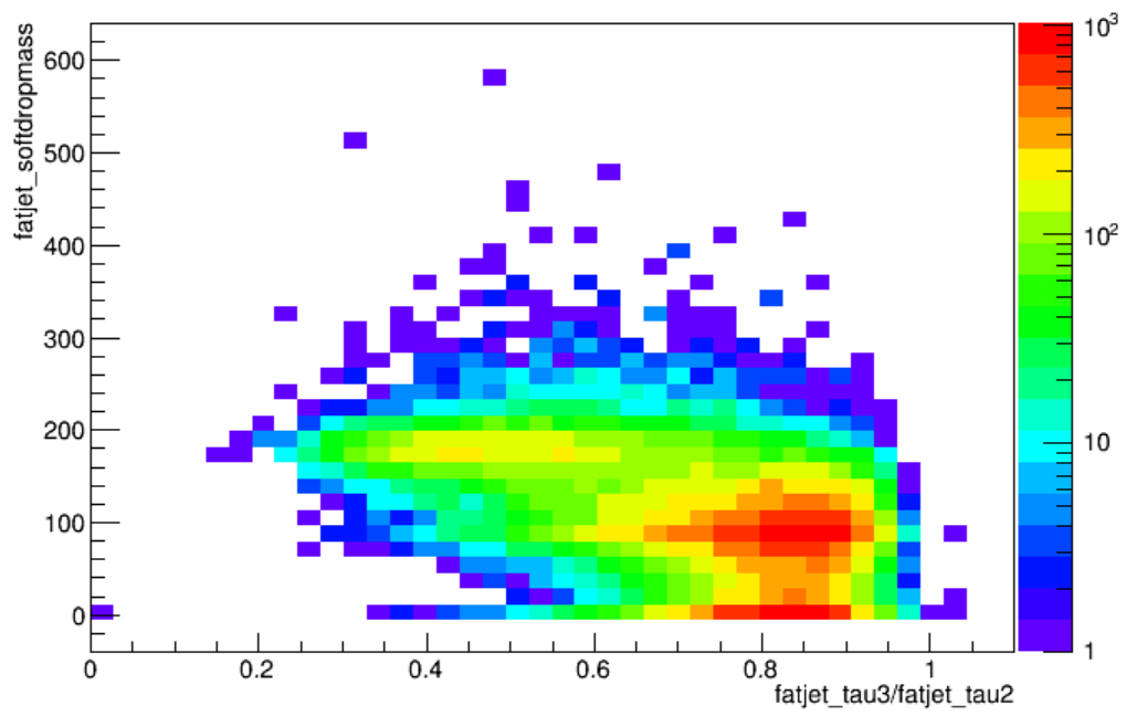
The figures below show the relevant tau ratios for W boson (left) and top quark (right) jets. The structure in the tau_2/tau_1 plot is very unique: W bosons pool at lower values of tau_2/tau_1, while top quarks (with more than 2 subjets) and light quarks (with only 1 subjet) pool at medium and higher values. In the tau_3/tau_2 plot, top quark jets have low values while both W boson and light quark jets are gathered near 1.
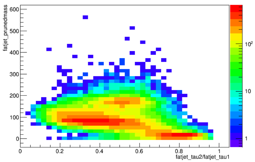 |
| 
For top quark or H boson decays, applying b tagging algorithms to the subjets of the large-radius jets gives another valuable substructure observable. The Combined Secondary Vertex v2 and the DeepCSV discriminants have been stored for the two subjets obtained from the soft drop algorithm in each large-radius jet. For simulation, we also store the generator-level flavor information for the subjet. You can explore the “Subjet” branches in NanoAOD here
Finally, NanoAOD contains some energy correlation function information for large-radius jets. The N2 and N3 functions are described in detail in a CMS paper on boosted jet identification.
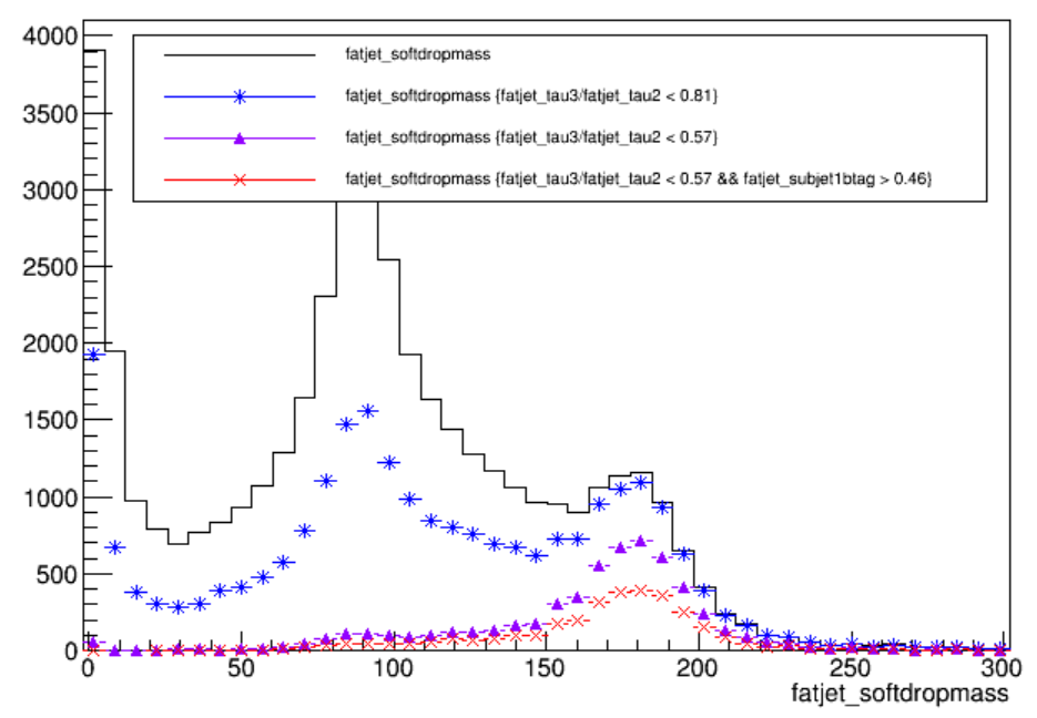
Groomed mass, jet substructure, and subjet b-tagging were the backbone of early boosted jet identification in CMS. The figure below shows an example of isolating top quark jets by applying various mass and substructure criteria. However, these algorithms have now been eclipsed by deep neural network identification techniques.
| Object property | Type | Description |
|---|---|---|
| FatJet_msoftdrop | Float_t | Corrected soft drop mass with PUPPI |
| FatJet_n2b1 | Float_t | N2 with beta=1 |
| FatJet_n3b1 | Float_t | N3 with beta=1 |
| FatJet_subJetIdx1 | Int_t | (index to Subjet) index of first subjet |
| FatJet_subJetIdx2 | Int_t | (index to Subjet) index of second subjet |
| FatJet_tau1 | Float_t | Nsubjettiness (1 axis) |
| FatJet_tau2 | Float_t | Nsubjettiness (2 axis) |
| FatJet_tau3 | Float_t | Nsubjettiness (3 axis) |
| FatJet_tau4 | Float_t | Nsubjettiness (4 axis) |
Deep Neural Network taggers
During Run 2, CMS analysts developed many neural network identification schemes for large-radius jets. The best performers have been preserved in the version of NanoAOD available for Open Data. The main algorithms are:
- DeepDoubleX (or “double-b”): a Boosted Decision Tree optimized for decays of massive particles to a pair of b or c quarks.
- DeepBoostedJet (or “DeepAK8”): a Convolutional Neural Network combined with a dense network that uses particle-flow candidates and secondary vertices to determine the parent particle of the jet
- ParticleNet: a Dynamic Graph Convolutional Neural Network applied on “point cloud” data structures built from the particle-flow candidates within a jet.
The deep network taggers provide discriminants for many different particle hypotheses. These are typically grouped into “binarized” discriminants intended to separate a particular massive particle (top, Higgs, etc) from light quark jets. Both DeepAK8 and ParticleNet offer “mass-decorrelated” discriminants, for which the network has been trained in such a way that jet mass is not part of the learning process. For analyses that use the jet mass distribution as a key sensitive variable, decorrelation helps maintain a smoothly falling light-quark jet mass distribution, with no artificial peak near the region of interest (eg, near 125 GeV for Higgs bosons, or new 170 GeV for top quarks).
The branches available in NanoAOD for the deep network taggers are listed below.
| Object property | Type | Description |
|---|---|---|
| FatJet_btagDDBvLV2 | Float_t | DeepDoubleX V2(mass-decorrelated) discriminator for H(Z)->bb vs QCD |
| FatJet_btagDDCvBV2 | Float_t | DeepDoubleX V2 (mass-decorrelated) discriminator for H(Z)->cc vs H(Z)->bb |
| FatJet_btagDDCvLV2 | Float_t | DeepDoubleX V2 (mass-decorrelated) discriminator for H(Z)->cc vs QCD |
| FatJet_btagHbb | Float_t | Higgs to BB tagger discriminator |
| FatJet_deepTagMD_H4qvsQCD | Float_t | Mass-decorrelated DeepBoostedJet tagger H->4q vs QCD discriminator |
| FatJet_deepTagMD_HbbvsQCD | Float_t | Mass-decorrelated DeepBoostedJet tagger H->bb vs QCD discriminator |
| FatJet_deepTagMD_TvsQCD | Float_t | Mass-decorrelated DeepBoostedJet tagger top vs QCD discriminator |
| FatJet_deepTagMD_WvsQCD | Float_t | Mass-decorrelated DeepBoostedJet tagger W vs QCD discriminator |
| FatJet_deepTagMD_ZHbbvsQCD | Float_t | Mass-decorrelated DeepBoostedJet tagger Z/H->bb vs QCD discriminator |
| FatJet_deepTagMD_ZHccvsQCD | Float_t | Mass-decorrelated DeepBoostedJet tagger Z/H->cc vs QCD discriminator |
| FatJet_deepTagMD_ZbbvsQCD | Float_t | Mass-decorrelated DeepBoostedJet tagger Z->bb vs QCD discriminator |
| FatJet_deepTagMD_ZvsQCD | Float_t | Mass-decorrelated DeepBoostedJet tagger Z vs QCD discriminator |
| FatJet_deepTagMD_bbvsLight | Float_t | Mass-decorrelated DeepBoostedJet tagger Z/H/gluon->bb vs light flavour discriminator |
| FatJet_deepTagMD_ccvsLight | Float_t | Mass-decorrelated DeepBoostedJet tagger Z/H/gluon->cc vs light flavour discriminator |
| FatJet_deepTag_H | Float_t | DeepBoostedJet tagger H(bb,cc,4q) sum |
| FatJet_deepTag_QCD | Float_t | DeepBoostedJet tagger QCD(bb,cc,b,c,others) sum |
| FatJet_deepTag_QCDothers | Float_t | DeepBoostedJet tagger QCDothers value |
| FatJet_deepTag_TvsQCD | Float_t | DeepBoostedJet tagger top vs QCD discriminator |
| FatJet_deepTag_WvsQCD | Float_t | DeepBoostedJet tagger W vs QCD discriminator |
| FatJet_deepTag_ZvsQCD | Float_t | DeepBoostedJet tagger Z vs QCD discriminator |
| FatJet_particleNetMD_QCD | Float_t | Mass-decorrelated ParticleNet tagger raw QCD score |
| FatJet_particleNetMD_Xbb | Float_t | Mass-decorrelated ParticleNet tagger raw X->bb score. For X->bb vs QCD tagging, use Xbb/(Xbb+QCD) |
| FatJet_particleNetMD_Xcc | Float_t | Mass-decorrelated ParticleNet tagger raw X->cc score. For X->cc vs QCD tagging, use Xcc/(Xcc+QCD) |
| FatJet_particleNetMD_Xqq | Float_t | Mass-decorrelated ParticleNet tagger raw X->qq (uds) score. For X->qq vs QCD tagging, use Xqq/(Xqq+QCD). For W vs QCD tagging, use (Xcc+Xqq)/(Xcc+Xqq+QCD) |
| FatJet_particleNet_H4qvsQCD | Float_t | ParticleNet tagger H(->VV->qqqq) vs QCD discriminator |
| FatJet_particleNet_HbbvsQCD | Float_t | ParticleNet tagger H(->bb) vs QCD discriminator |
| FatJet_particleNet_HccvsQCD | Float_t | ParticleNet tagger H(->cc) vs QCD discriminator |
| FatJet_particleNet_QCD | Float_t | ParticleNet tagger QCD(bb,cc,b,c,others) sum |
| FatJet_particleNet_TvsQCD | Float_t | ParticleNet tagger top vs QCD discriminator |
| FatJet_particleNet_WvsQCD | Float_t | ParticleNet tagger W vs QCD discriminator |
| FatJet_particleNet_ZvsQCD | Float_t | ParticleNet tagger Z vs QCD discriminator |
| FatJet_particleNet_mass | Float_t | ParticleNet mass regression |
Tagger scale factors
Scale factors to increase or decrease the number of tagged jets in simulation can be applied in a number of ways, but typically involve weighting simulation events based on the efficiencies and scale factors relevant to each jet in the event.
For small-radius jet b-tagging, details and usage references from Run 1 can be found at these references. The concepts and methods for applying scale factors are unchanged in Run 2.
The most common scale factor application method (1a) relies on 4
pieces of information for each jet in simulation: * Tagging status: does
this jet pass the discriminator threshold for a given working point? *
Flavor (b, c, light): accessed using a pat::Jet member
function called partonFlavour(). * Efficiency: measured as
a function of momentum as in the image above. * Scale factor: accessed
from the
For large-radius jet tagging, scale factors are computed for specific boosted particle flavors and can be applied using similar methods as for b tagging.
Spplication instructions coming soon!
The CMS Open Data Guide will include the scale factor data files and application instructions for 2015 and 2016 Open Data.
Key Points
- Tagging algorithms separate heavy flavor jets from jets produced by the hadronization of light quarks and gluons
- FatJet tagging algorithms can identify jets from massive SM particles
- Tagging algorithms produce a disriminator value for each jet that represents the likelihood that the jet came from a particular particle
- Each tagging algorithm has recommended ‘working points’ (discriminator values) based on a misidentification probability for non-interesting jets