Pre-lesson reading and computational setup
Overview
Teaching: 30 min
Exercises: 20 minQuestions
What analysis will we be doing?
Objectives
Skim the paper on which this lesson is based.
Make sure your computing environment is setup properly
Physics introduction
In this lesson, you will be walked through a mini-reproduction of a 2017 analysis from the CMS collaboration. The cross-section for the production of top-quark / anti-top-quark pairs in proton-proton collisions was measured. Put another way, we measured the probability that a top-quark and an anti-top quark pair are produced when protons are collided at a center-of-mass energy of 13 TeV.
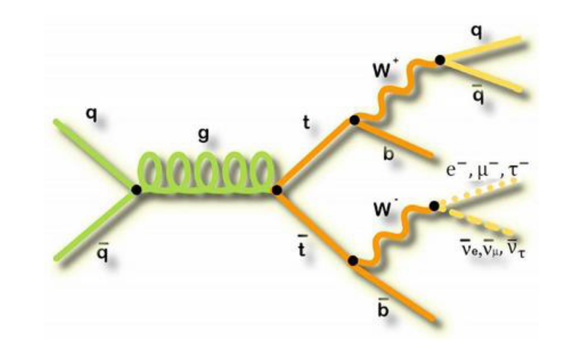 .
.
To go into a bit more detail in this simplified analysis we will be working towards a measurement of the top and anti-top quark production cross section \(\sigma_{t\bar{t}}\). The data are produced in proton-proton collisions at \(\sqrt{s}\) = 13 TeV at the beginning of Run 2 of the LHC. We will be examining the lepton+jets final state \(t\bar{t} \rightarrow (bW^{+})(\bar{b}W_{-}) \rightarrow bq\bar{q} bl^{-}\bar{\nu_{l}}\) which is characterized by one lepton (here we look at electrons and muons only), significant missing transverse energy, and four jets, two of which are identified as b-jets.
Depending on how much background you have, try to read or at least skim the paper and see how much you can get out of it. We’ll discuss it in more detail in our first episode when we meet.
Set up your computing environment.
We will attempt to use tools that are built on modern, powerful and efficient python ecosystems. In particular, we will use the Columnar Object Framework For Effective Analysis (Coffea), which will provide us with basic tools and wrappers for enabling not-too-alien syntax when running columnar Collider HEP analysis.
Start up Docker and JupyterLab
Type out the following commands for this episode!
For this next section, you’ll be asked to type out the provided commands in a Jupyter notebook, a popular development environment that allows you to use python in an interactive way.
Please enter in these commands yourself for this episode.
To create or run these notebooks, we will
- Start the python docker container
- Install some necessary extra module (this only needs to be done once)
- Launch Jupyter Lab, an application that makes it easier to work with Jupyter Notebooks
- Create a new Jupyter Notebook for this episode.
Start Docker If you have already successfully installed and run the Docker example with python tools, then you need only execute the following command.
docker start -i my_python #give the name of your container
If this doesn’t work, return to the python tools Docker container lesson to work through how to start the container.
Install the extra libraries
(If you did this already by following the setup section of this lesson, then you needn’t do this part again.)
In order to use the coffea framework for our analysis, we need to install these additional packages directly in our container. We are adding
cabinetry as well because we will use it later in our last episode. This can take a few minutes to install.
pip install vector hist mplhep coffea cabinetry
Also, download this file, which is our starting schema. Directly in your /code area (or locally in your cms_open_data_python directory) you can simply do:
wget https://raw.githubusercontent.com/cms-opendata-workshop/workshop2022-lesson-ttbarljetsanalysis-payload/master/trunk/agc_schema.py
Launch Jupyter Lab In your docker python container, type the following.
jupyter-lab --ip=0.0.0.0 --no-browser
Launching Jupyter Lab
You should see something like this in your Docker container terminal when you type the above
jupyter-labcommand.
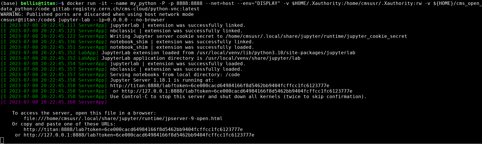
In the image above you can see the output when I start jupyter-lab on my computer. Yours won’t say exactly
the same thing, but it should be similar. Take note of the last two lines that start with http://. Start up a
browser locally on your laptop or desktop (not from the Docker container). Copy one of those
URLs and paste it into the browser. If the first URL doesn’t work, try the other.
If it works you’ll see something in your browser similar to the following image!
Launching Jupyter Lab
If Jupyter Lab launched, you’ll see something like this.
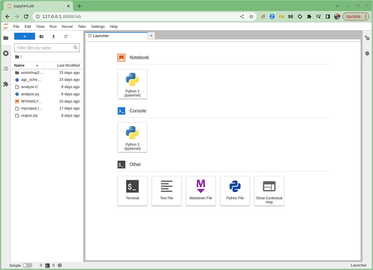
Great! You’re all set to begin the analysis!
Key Points
Get ready for the lesson as a whole
Introduction
Overview
Teaching: 20 min
Exercises: 20 minQuestions
What analysis will we be doing?
What is columnar analysis?
Why do we use coffea?
What are coffea main components?
What are schemas?
Objectives
Learn about the physics behind the analysis example.
Learn about the strategy we will follow for our analysis example.
Learn what the difference is between columnar and loop analysis.
Learn what coffea is and what the logic is of its different compoonets
Learn about what schemas are used for and how to modify them
Physics introduction
In this lesson, you will be walked through a mini-reproduction of a 2017 analysis from the CMS collaboration. The cross-section for the production of top-quark / anti-top-quark pairs in proton-proton collisions was measured. Put another way, we measured the probability that a top-quark and an anti-top quark pair are produced when protons are collided at a center-of-mass energy of 13 TeV.
.
To go into a bit more detail
in this simplified analysis we will be working towards a measurement of the top and anti-top quark production cross section \(\sigma_{t\bar{t}}\).
The data are produced in proton-proton collisions at \(\sqrt{s}\) = 13 TeV at the beginning of Run 2 of the LHC. We will be examining the lepton+jets final state
\(t\bar{t} \rightarrow (bW^{+})(\bar{b}W_{-}) \rightarrow bq\bar{q} bl^{-}\bar{\nu_{l}}\)
which is characterized by one lepton (here we look at electrons and muons only), significant missing transverse energy, and four jets, two of which are identified as b-jets.
Slides
We want to motivate why we are encouraging you to look into some of these newer software tools. Let’s go through these slides together to review this analysis and to get a more complete overview of what goes into an analysis.
Coding (python) introduction
We will attempt to use tools that are built on modern, powerful and efficient python ecosystems. In particular, we will use the Columnar Object Framework For Effective Analysis (Coffea), which will provide us with basic tools and wrappers for enabling not-too-alien syntax when running columnar Collider HEP analysis.
Start up Docker and JupyterLab
Type out the following commands for this episode!
For this next section, you’ll be asked to type out the provided commands in a Jupyter notebook, a popular development environment that allows you to use python in an interactive way.
Please enter in these commands yourself for this episode.
To create or run these notebooks, we will
- Start the python docker container
- Install some necessary extra module (this only needs to be done once)
- Launch Jupyter Lab, an application that makes it easier to work with Jupyter Notebooks
- Create a new Jupyter Notebook for this episode.
Start Docker If you have already successfully installed and run the Docker example with python tools, then you need only execute the following command.
docker start -i my_python #give the name of your container
If this doesn’t work, return to the python tools Docker container lesson to work through how to start the container.
Install the extra libraries
(If you did this already by following the setup section of this lesson, then you needn’t do this part again.)
In order to use the coffea framework for our analysis, we need to install these additional packages directly in our container. We are adding
cabinetry as well because we will use it later in our last episode. This can take a few minutes to install.
pip install vector hist mplhep coffea cabinetry
Also, download this file, which is our starting schema. Directly in your /code area (or locally in your cms_open_data_python directory) you can simply do:
wget https://raw.githubusercontent.com/cms-opendata-workshop/workshop2022-lesson-ttbarljetsanalysis-payload/master/trunk/agc_schema.py
Launch Jupyter Lab In your docker python container, type the following.
jupyter-lab --ip=0.0.0.0 --no-browser
Launching Jupyter Lab
You should see something like this in your Docker container terminal when you type the above
jupyter-labcommand.
In the image above you can see the output when I start jupyter-lab on my computer. Yours won’t say exactly
the same thing, but it should be similar. Take note of the last two lines that start with http://. Start up a
browser locally on your laptop or desktop (not from the Docker container). Copy one of those
URLs and paste it into the browser. If the first URL doesn’t work, try the other.
If it works you’ll see something in your browser similar to the following image!
Launching Jupyter Lab
If Jupyter Lab launched, you’ll see something like this.
Start a new Jupyter notebook
The top icon (under Notebook) says Python 3 (ipykernel). Click on this icon. This should launch a new Jupyter notebook!
Starting a new Jupyter notebook
If your new Jupyter Notebook started, you’ll see something like this.

In this Jupyter Lab environment, click on File (in the top right) and then from the dropdown
menu select Rename Notebook…. You can call this notebook whatever you like but I have
called mine analysis_example_prelesson.ipynb.
For the remainder of this lesson, you’ll be typing or cutting-and-pasting the commands you see here in the Python sections into the Jupyter Notebook. To run those commands after you have typed them, you can press the little Play icon (right-pointing triangle) or type Shift + Enter (to run the cell and advance) or Ctrl + Enter (to run the cell and not advance). Whichever you prefer.
Optional! Using ipython
If, for some reason, you don’t want to use Jupyter, you can launch interactive python just by typing
ipythonin Docker Container (and not thejupyter-labcommand) and then entering the python commands there.
Columnar analysis basics with Awkward
Note: this and the next section on this episode are a recast (with some shameless copying and pasting) of this notebook by Mat Adamec presented during the IRIS-HEP AGC Workshop 2022.
In one of the pre-exercises we learned how to access ROOT files (the standard use at the LHC experiments) using uproot and why the awkward library can be very helpufl when dealing with jagged arrays.
Let’s remember very quickly. First, be sure to import the appropriate libraries:
import uproot
import awkward as ak
Let’s open an example file. These are flattened POET ntuples. As it was mentioned in the trigger lesson, we will be producing these skimmed ntuples for you. You may recognize all the variables we had worked with before.
Using uproot,
events = uproot.open('root://eospublic.cern.ch//eos/opendata/cms/upload/od-workshop/ws2021/myoutput_odws2022-ttbaljets-prodv2.0_merged.root')['events']
events
<TTree 'events' (275 branches) at 0x7fb46a8b5870>.
We now have an events tree. We can view its branches by querying its keys():
events.keys()
['numberelectron', 'nelectron_e', 'electron_e', 'nelectron_pt', 'electron_pt', 'nelectron_px', 'electron_px', 'nelectron_py', 'electron_py', 'nelectron_pz', 'electron_pz', 'nelectron_eta', 'electron_eta', 'nelectron_phi', 'electron_phi', 'nelectron_ch', 'electron_ch', 'nelectron_iso', 'electron_iso', 'nelectron_veto', 'electron_veto', 'nelectron_isLoose', 'electron_isLoose', 'nelectron_isMedium', 'electron_isMedium', 'nelectron_isTight', 'electron_isTight', 'nelectron_dxy', 'electron_dxy', 'nelectron_dz', 'electron_dz', 'nelectron_dxyError', 'electron_dxyError', 'nelectron_dzError', 'electron_dzError', 'nelectron_ismvaLoose', 'electron_ismvaLoose', 'nelectron_ismvaTight', 'electron_ismvaTight', 'nelectron_ip3d', 'electron_ip3d', 'nelectron_sip3d', 'electron_sip3d', 'numberfatjet', 'nfatjet_e', 'fatjet_e', 'nfatjet_pt', 'fatjet_pt', 'nfatjet_eta', 'fatjet_eta', 'nfatjet_phi', 'fatjet_phi', 'nfatjet_ch', 'fatjet_ch', 'nfatjet_mass', 'fatjet_mass', 'nfatjet_corrpt', 'fatjet_corrpt', 'nfatjet_corrptUp', 'fatjet_corrptUp', 'nfatjet_corrptDown', 'fatjet_corrptDown', 'nfatjet_corrptSmearUp', 'fatjet_corrptSmearUp', 'nfatjet_corrptSmearDown', 'fatjet_corrptSmearDown', 'nfatjet_corrmass', 'fatjet_corrmass', 'nfatjet_corre', 'fatjet_corre', 'nfatjet_corrpx', 'fatjet_corrpx', 'nfatjet_corrpy', 'fatjet_corrpy', 'nfatjet_corrpz', 'fatjet_corrpz', 'nfatjet_prunedmass', 'fatjet_prunedmass', 'nfatjet_softdropmass', 'fatjet_softdropmass', 'nfatjet_tau1', 'fatjet_tau1', 'nfatjet_tau2', 'fatjet_tau2', 'nfatjet_tau3', 'fatjet_tau3', 'nfatjet_subjet1btag', 'fatjet_subjet1btag', 'nfatjet_subjet2btag', 'fatjet_subjet2btag', 'nfatjet_subjet1hflav', 'fatjet_subjet1hflav', 'nfatjet_subjet2hflav', 'fatjet_subjet2hflav', 'numberjet', 'njet_e', 'jet_e', 'njet_pt', 'jet_pt', 'njet_eta', 'jet_eta', 'njet_phi', 'jet_phi', 'njet_ch', 'jet_ch', 'njet_mass', 'jet_mass', 'njet_btag', 'jet_btag', 'njet_hflav', 'jet_hflav', 'njet_corrpt', 'jet_corrpt', 'njet_corrptUp', 'jet_corrptUp', 'njet_corrptDown', 'jet_corrptDown', 'njet_corrptSmearUp', 'jet_corrptSmearUp', 'njet_corrptSmearDown', 'jet_corrptSmearDown', 'njet_corrmass', 'jet_corrmass', 'njet_corre', 'jet_corre', 'njet_corrpx', 'jet_corrpx', 'njet_corrpy', 'jet_corrpy', 'njet_corrpz', 'jet_corrpz', 'btag_Weight', 'btag_WeightUp', 'btag_WeightDn', 'met_e', 'met_pt', 'met_px', 'met_py', 'met_phi', 'met_significance', 'met_rawpt', 'met_rawphi', 'met_rawe', 'numbermuon', 'nmuon_e', 'muon_e', 'nmuon_pt', 'muon_pt', 'nmuon_px', 'muon_px', 'nmuon_py', 'muon_py', 'nmuon_pz', 'muon_pz', 'nmuon_eta', 'muon_eta', 'nmuon_phi', 'muon_phi', 'nmuon_ch', 'muon_ch', 'nmuon_isLoose', 'muon_isLoose', 'nmuon_isMedium', 'muon_isMedium', 'nmuon_isTight', 'muon_isTight', 'nmuon_isSoft', 'muon_isSoft', 'nmuon_isHighPt', 'muon_isHighPt', 'nmuon_dxy', 'muon_dxy', 'nmuon_dz', 'muon_dz', 'nmuon_dxyError', 'muon_dxyError', 'nmuon_dzError', 'muon_dzError', 'nmuon_pfreliso03all', 'muon_pfreliso03all', 'nmuon_pfreliso04all', 'muon_pfreliso04all', 'nmuon_pfreliso04DBCorr', 'muon_pfreliso04DBCorr', 'nmuon_TkIso03', 'muon_TkIso03', 'nmuon_jetidx', 'muon_jetidx', 'nmuon_genpartidx', 'muon_genpartidx', 'nmuon_ip3d', 'muon_ip3d', 'nmuon_sip3d', 'muon_sip3d', 'numberphoton', 'nphoton_e', 'photon_e', 'nphoton_pt', 'photon_pt', 'nphoton_px', 'photon_px', 'nphoton_py', 'photon_py', 'nphoton_pz', 'photon_pz', 'nphoton_eta', 'photon_eta', 'nphoton_phi', 'photon_phi', 'nphoton_ch', 'photon_ch', 'nphoton_chIso', 'photon_chIso', 'nphoton_nhIso', 'photon_nhIso', 'nphoton_phIso', 'photon_phIso', 'nphoton_isLoose', 'photon_isLoose', 'nphoton_isMedium', 'photon_isMedium', 'nphoton_isTight', 'photon_isTight', 'nPV_chi2', 'PV_chi2', 'nPV_ndof', 'PV_ndof', 'PV_npvs', 'PV_npvsGood', 'nPV_x', 'PV_x', 'nPV_y', 'PV_y', 'nPV_z', 'PV_z', 'trig_Ele22_eta2p1_WPLoose_Gsf', 'trig_IsoMu20', 'trig_IsoTkMu20', 'numbertau', 'ntau_e', 'tau_e', 'ntau_pt', 'tau_pt', 'ntau_px', 'tau_px', 'ntau_py', 'tau_py', 'ntau_pz', 'tau_pz', 'ntau_eta', 'tau_eta', 'ntau_phi', 'tau_phi', 'ntau_ch', 'tau_ch', 'ntau_mass', 'tau_mass', 'ntau_decaymode', 'tau_decaymode', 'ntau_iddecaymode', 'tau_iddecaymode', 'ntau_idisoraw', 'tau_idisoraw', 'ntau_idisovloose', 'tau_idisovloose', 'ntau_idisoloose', 'tau_idisoloose', 'ntau_idisomedium', 'tau_idisomedium', 'ntau_idisotight', 'tau_idisotight', 'ntau_idantieletight', 'tau_idantieletight', 'ntau_idantimutight', 'tau_idantimutight']
Each of these branches can be interpreted as an awkward array. Let’s examine their contents to remember that they contain jagged (non-rectangular) arrays:
muon_pt = events['muon_pt'].array()
print(muon_pt)
[[53.4, 0.792], [30.1], [32.9, 0.769, 0.766], ... 40], [37.9], [35.2], [30.9, 3.59]]
We could get the number of muons in each collision with:
ak.num(muon_pt, axis=-1)
<Array [2, 1, 3, 1, 1, 1, ... 1, 1, 1, 1, 1, 2] type='15090 * int64'>
A quick note about axes in awkward: 0 is always the shallowest, while -1 is the deepest. In other words, axis=0 would tell us the number of subarrays (events), while axis=-1 would tell us the number of muons within each subarray. This array is only of dimension 2, so axis=1 or axis=-1 are the same. This usage is the same as for standard numpy arrays.
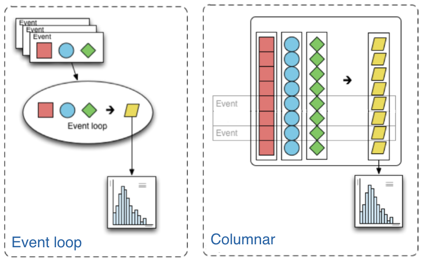
The traditional way of analyzing data in HEP involves the event loop. In this paradigm, we would write an explicit loop to go through every event (and through every field of an event that we wish to make a cut on). This method of analysis is rather bulky in comparison to the columnar approach, which (ideally) has no explicit loops at all! Instead, the fields of our data are treated as arrays and analysis is done by way of numpy-like array operations.
Most simple cuts can be handled by masking. A mask is a Boolean array which is generated by applying a condition to a data array. For example, if we want only muons with pT > 10, our mask would be:
print(muon_pt > 10)
[[True, False], [True], [True, False, False], ... [True], [True], [True, False]]
Then, we can apply the mask to our data. The syntax follows other standard array selection operations: data[mask]. This will pick out only the elements of our data which correspond to a True.
Our mask in this case must have the same shape as our muons branch, and this is guaranteed to be the case since it is generated from the data in that branch. When we apply this mask, the output should have the same amount of events, but it should down-select muons - muons which correspond to False should be dropped. Let’s compare to check:
print('Input:', muon_pt)
print('Output:', muon_pt[muon_pt > 10])
Input: [[53.4, 0.792], [30.1], [32.9, 0.769, 0.766], ... 40], [37.9], [35.2], [30.9, 3.59]]
Output: [[53.4], [30.1], [32.9], [28.3], [41.7], ... [42.6], [40], [37.9], [35.2], [30.9]]
We can also confirm we have fewer muons now, but the same amount of events:
print('Input Counts:', ak.sum(ak.num(muon_pt, axis=1)))
print('Output Counts:', ak.sum(ak.num(muon_pt[muon_pt > 10], axis=1)))

print('Input Size:', ak.num(muon_pt, axis=0))
print('Output Size:', ak.num(muon_pt[muon_pt > 10], axis=0))
Input Counts: 26690
Output Counts: 17274

Input Size: 15090
Output Size: 15090
Challenge!
How many muons have a transverse momentum (
pt) greater than 30 GeV/c?Revisit the output of
event.keys(). How many jets in total were produced and how many have a transverse momentum greater than 30 GeV/c?Solution
We modify the above code to mask the muons with
muon_pt> 30. We also make use of thejet_ptvariable to perform a similar calculation.print('Input Counts:', ak.sum(ak.num(muon_pt, axis=1))) print('Output Counts:', ak.sum(ak.num(muon_pt[muon_pt > 30], axis=1)))Input Counts: 26690 Output Counts: 13061jet_pt = events['jet_pt'].array() print('Input Counts:', ak.sum(ak.num(jet_pt, axis=1))) print('Output Counts:', ak.sum(ak.num(jet_pt[jet_pt > 30], axis=1))) print('Input Counts:', ak.num(jet_pt, axis=0)) print('Output Counts:', ak.num(jet_pt[jet_pt > 30], axis=0))Input Counts: 26472 Output Counts: 19419 Input Counts: 15090 Output Counts: 15090So we find that there are 13061 muons, taken from these 15090 proton-proton collisions that have transverse momentum greater than 30 GeV/c.
Similarly we find that there are 26472 jets, taken from these 15090 proton-proton collisions, and 19419 of them have transverse momentum greater than 30 GeV/c.
Let’s quickly make a simple histogram with the widely used matplotlib library. First we will import it.
import matplotlib.pylab as plt
When we make our histogram, we need to first “flatten” the awkward aray before passing it to matplotlib.
This is because matplotlib doesn’t know how to handle the jagged nature of awkward arrays.
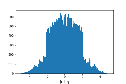
# Flatten the jagged array before we histogram it
values = ak.flatten(events['jet_eta'].array())

fig = plt.figure(figsize=(6,4))
plt.hist(values,bins=100,range=(-5,5))
plt.xlabel(f'Jet $\eta$',fontsize=14)
;
(The semi-colon at the end of the code is just to suppress the output of whatever the last line of the python code in the cell.)
Output of
jet_etahistogram
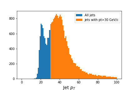
And here’s how we could use the mask in our plot.
# Flatten the jagged array before we histogram it
fig = plt.figure(figsize=(6,4))

values = ak.flatten(jet_pt)

plt.hist(values,bins=100,range=(0,100), label='All jets')
plt.hist(values[values>30],bins=100,range=(0,100), label='jets with pt>30 GeV/c')

plt.xlabel(f'Jet $p_T$',fontsize=14)
plt.legend()
;
Output of
jet_pthistogram with and without mask
Coffea
Awkward arrays let us access data in a columnar fashion, but that’s just the first part of doing an analysis. Coffea builds upon this foundation with a variety of features that better enable us to do our analyses. These features include:
-
Hists give us ROOT-like histograms. Actually, this is now a standalone package, but it has been heavily influenced by the (old) coffea hist subpackage, and it’s a core component of the coffea ecosystem.
-
NanoEvents and Schemas allows us to apply a schema to our awkward array. This schema imposes behavior that we would not have in a simple awkward array, but which makes our (HEP) lives much easier. On one hand, it can serve to better organize our data by providing a structure for naming, nesting, and cross-referencing fields; it also allows us to add physics object methods (e.g., for LorentzVectors).
-
Processors are coffea’s way of encapsulating an analysis in a way that is deployment-neutral. Once you have a Coffea analysis, you can throw it into a processor and use any of a variety of executors (e.g. Dask, Parsl, Spark) to chunk it up and run it across distributed workers. This makes scale-out simple and dynamic for users.
-
Lookup tools are available in Coffea for any corrections that need to be made to physics data. These tools read a variety of correction file formats and turn them into lookup tables.
In summary, coffea’s features enter the analysis pipeline at every step. They improve the usability of our input (NanoEvents), enable us to map it to a histogram output (Hists), and allow us tools for scaling and deployment (Processors).
Coffea NanoEvents and Schemas: Making Data Physics-Friendly
Before we can dive into our example analysis, we need to spruce up our data a bit.
Let’s turn our attention to NanoEvents and schemas. Schemas let us better organize our file and impose physics methods onto our data. There exist schemas for some standard file formats, most prominently NanoAOD (which will be, in the future, the main format in which CMS data will be made open), and there is a BaseSchema which operates much like uproot. The coffea development team welcomes community development of other schemas.
For the purposes of this tutorial, we already have a schema. Again, this was prepared already by Mat Adamec for the IRIS-HEP AGC Workshop 2022. Here, however, we will try to go into the details.
Before we start, don’t forget to include the libraries we need, including now the coffea ones:
import uproot
import awkward as ak
import hist
from hist import Hist
from coffea.nanoevents import NanoEventsFactory, BaseSchema
Remember the output we had above. After loading the file, we saw a lot of branches. Let’s zoom in on the muon-related ones here:
'numbermuon', 'nmuon_e', 'muon_e', 'nmuon_pt', 'muon_pt', 'nmuon_px', 'muon_px', 'nmuon_py', 'muon_py', 'nmuon_pz', 'muon_pz', 'nmuon_eta', 'muon_eta', 'nmuon_phi', 'muon_phi', 'nmuon_ch', 'muon_ch', 'nmuon_isLoose', 'muon_isLoose', 'nmuon_isMedium', 'muon_isMedium', 'nmuon_isTight', 'muon_isTight', 'nmuon_isSoft', 'muon_isSoft', 'nmuon_isHighPt', 'muon_isHighPt', 'nmuon_dxy', 'muon_dxy', 'nmuon_dz', 'muon_dz', 'nmuon_dxyError', 'muon_dxyError', 'nmuon_dzError', 'muon_dzError', 'nmuon_pfreliso03all', 'muon_pfreliso03all', 'nmuon_pfreliso04all', 'muon_pfreliso04all', 'nmuon_pfreliso04DBCorr', 'muon_pfreliso04DBCorr', 'nmuon_TkIso03', 'muon_TkIso03', 'nmuon_jetidx', 'muon_jetidx', 'nmuon_genpartidx', 'muon_genpartidx', 'nmuon_ip3d', 'muon_ip3d', 'nmuon_sip3d', 'muon_sip3d'
By default, uproot (and BaseSchema) treats all of the muon branches as distinct branches with distinct data. This is not ideal, as some of our data is redundant, e.g., all of the nmuon_* branches better have the same counts. Further, we’d expect all the muon_* branches to have the same shape, as each muon should have an entry in each branch.
The first benefit of instating a schema, then, is a standardization of our fields. It would be more succinct to create a general muon collection under which all of these branches (in NanoEvents, fields) with identical size can be housed, and to scrap the redundant ones. We can use numbermuon to figure out how many muons should be in each subarray (the counts, or offsets), and then fill the contents with each muon_* field. We can repeat this for the other branches.
We will, however, use a custom schema called AGCSchema, whose implementation resides in the agc_schema.py file you just downloaded.
Let’s open our example file again, but now, instead of directly using uproot, we use the AGCSchema class.
from agc_schema import AGCSchema
agc_events = NanoEventsFactory.from_root('root://eospublic.cern.ch//eos/opendata/cms/upload/od-workshop/ws2021/myoutput_odws2022-ttbaljets-prodv2.0_merged.root', schemaclass=AGCSchema, treepath='events').events()
For NanoEvents, there is a slightly different syntax to access our data. Instead of querying keys() to find our fields, we query fields. We can still access specific fields as we would navigate a dictionary (collection[field]) or we can navigate them in a new way: collection.field.
Let’s take a look at our fields now:
agc_events.fields
['muon', 'fatjet', 'jet', 'photon', 'electron', 'tau', 'met', 'trig', 'btag', 'PV']
We can confirm that no information has been lost by querying the fields of our event fields:
agc_events.muon.fields
['pt', 'px', 'py', 'pz', 'eta', 'phi', 'ch', 'isLoose', 'isMedium', 'isTight', 'isSoft', 'isHighPt', 'dxy', 'dz', 'dxyError', 'dzError', 'pfreliso03all', 'pfreliso04all', 'pfreliso04DBCorr', 'TkIso03', 'jetidx', 'genpartidx', 'ip3d', 'sip3d', 'energy']
So, aesthetically, everything is much nicer. If we had a messier dataset, the schema can also standardize our names to get rid of any quirks. For example, every physics object property in our tree has an n* variable which, if you were to check their values, you would realize that they repeat. They give just the number of objects in the field. We need only one variable to check that, and for the muons would be numbermuon. This sort of features are irrelevant after the application of the schema, so we don’t have to worry about it.
There are also other benefits to this structure: as we now have a collection object (agc_events.muon), there is a natural place to impose physics methods. By default, this collection object does nothing - it’s just a category. But we’re physicists, and we often want to deal with Lorentz vectors. Why not treat these objects as such?
This behavior can be built fairly simply into a schema by specifying that it is a PtEtaPhiELorentzVector and having the appropriate fields present in each collection (in this case, pt, eta, phi and e). This makes mathematical operations on our muons well-defined:
agc_events.muon[0, 0] + agc_events.muon[0, 1]
<LorentzVectorRecord ... y: -17.7, z: -11.9, t: 58.2} type='LorentzVector["x": f...'>
And it gives us access to all of the standard LorentzVector methods, like \(\Delta R\):
agc_events.muon[0, 0].delta_r(agc_events.muon[0, 1])
2.512794926098977
We can also access other LorentzVector formulations, if we want, as the conversions are built-in:
agc_events.muon.x, agc_events.muon.y, agc_events.muon.z, agc_events.muon.mass
/usr/local/venv/lib/python3.10/site-packages/awkward/_connect/_numpy.py:195: RuntimeWarning: invalid value encountered in sqrt
  result = getattr(ufunc, method)(
(<Array [[50.7, 0.0423], ... [21.1, -1.38]] type='15090 * var * float32'>, <Array [[-16.9, -0.791], ... [-22.6, 3.31]] type='15090 * var * float32'>, <Array [[-7.77, -4.14], ... [-11, -6.83]] type='15090 * var * float32'>, <Array [[0.103, 0.106], ... [0.105, 0.106]] type='15090 * var * float32'>)
NanoEvents can also impose other features, such as cross-references in our data; for example, linking the muon jetidx to the jet collection. This is not implemented in our present schema.
Let’s take a look at the agc_schema.py file
Anyone, in principle, can write a schema that suits particular needs and that could be plugged into the coffea insfrastructure. Here we present a challenge to give you a feeling of the kind of arrangements schemas can take care of.
Challenge: Finding the corrected jet energy in the LorentzVector
If you check the variables above, you will notice that the
jetobject has an energyerecorded but also, as you learn from the physics objects lesson,corre, which is the corrected energy. You can also realize about this if you dump the fields for the jet:agc_events.jet.fieldsYou should find that you can see the
correvariable.Inspect and study the file
agc_schema.pyto see how thecorreenergy was added as the energy to the LorentzVector and not the uncorrectedeenergy. The changes for_eshould remain valid for the rest of the objects though. Note that you could correct for thefatjetalso in the same line of action.
Overnight challenge! Make your own plot!
You’ve now seen how to make basic plots of the variables in these ROOT files, as well as how to mask the data based on other variables.
You are challenged to make at least one plot, making use of the data file and tools we learned about in this lesson. It doesn’t matter what it is…you can even just reproduce the plots we asked you to make in this lesson. To save the plot, you’ll want to add something like the following line of code after you make any of the plots.
plt.savefig('my_plot.png')The figure will show up in the directory in both docker and on your local machine.
When you get the image, you can add it to these Google Slides.
Good luck! And we’ll pick this up tomorrow!
Key Points
Understanding the basic physics will help you understand how to translate physics into computer code.
We will be perfoming a real but simplified HEP analysis using CMS Run2 open data using columnar analysis.
Coffea is a framework which builds upons several tools to make columnar analysis more efficient in HEP.
Schemas are a simple way of rearranging our data content so it is easier to manipulate
Coffea Analysis
Overview
Teaching: 20 min
Exercises: 60 minQuestions
What is the general plan for the analysis?
What are the selection requirements?
How do I implement additional selection requirements?
What are Coffea Processors?
How do I run an analysis with Coffea?
Objectives
Understand the general strategy for the analysis
Learn how implement basic selection requirements
Learn how to build Coffea Processors and run an analysis
Getting things prepared for this episode
I’m going to assume that you have stopped the Docker container from the last episode. If you have not, let’s walk through how to start things up and add one more piece of data.
Type out the following commands for this episode!
For this next section, you’ll be asked to type out the provided commands in a Jupyter notebook, a popular development environment that allows you to use python in an interactive way.
Please enter in these commands yourself for this episode.
To create or run the notebooks used in this episode, we will
- Start the python docker container
- We assume that we have installed the necessary modules from the previous episode (e.g.
coffea)
- We assume that we have installed the necessary modules from the previous episode (e.g.
- Clone a repository of some helpful utilities for this episode.
- Launch Jupyter Lab.
- Create a new Jupyter Notebook for this episode.
Start Docker If you have already successfully installed and run the Docker example with python tools, then you need only execute the following command.
docker start -i my_python #give the name of your container
If this doesn’t work, return to the python tools Docker container lesson to work through how to start the container.
Clone a new repository
In your python Docker container clone the repository for this exercise and go into the cloned directory.
git clone https://github.com/cms-opendata-workshop/workshop2022-lesson-ttbarljetsanalysis-payload.git

cd workshop2022-lesson-ttbarljetsanalysis-payload
Launch Jupyter Lab In your docker python container, type the following.
jupyter-lab --ip=0.0.0.0 --no-browser
Take note of the last two lines that start with http://. Start up a
browser locally on your laptop or desktop (not from the Docker container). Copy one of those
URLs and paste it into the browser. If the first URL doesn’t work, try the other.
Start a new Jupyter notebook
The top icon (under Notebook) says Python 3 (ipykernel). Click on this icon. This should launch a new Jupyter notebook!
In this Jupyter Lab environment, click on File (in the top right) and then from the dropdown
menu select Rename Notebook…. You can call this notebook whatever you like but I have
called mine ttbar_analysis.ipynb.
For the remainder of this lesson, you’ll be typing or cutting-and-pasting the commands you see here in the Python sections into the Jupyter Notebook. To run those commands after you have typed them, you can press the little Play icon (right-pointing triangle) or type Shift + Enter (to run the cell and advance) or Ctrl + Enter (to run the cell and not advance). Whichever you prefer.
Optional! Using ipython
If, for some reason, you don’t want to use Jupyter, you can launch interactive python just by typing
ipythonin Docker Container (and not thejupyter-labcommand) and then entering the python commands there.
The analysis
This episode is a recast of the analysis demo presented by Alexander Held at the IRIS-HEP AGC Workshop 2022. Our attempt is to make it more understandable by paying a bit more attention to the details. Note that this is work in progress and it will be refined in the future, perhaps using better consolidated ntuples (nanoAOD-like).
Datasets and pre-selection
As it was mentioned in the previous episode, we will be working towards a measurement of the top and anti-top quark production cross section \(\sigma_{t\bar{t}}\).
The \(t\bar{t}\) pair is identified in a particular decay mode referred to as the lepton+jets final state.
[\begin{eqnarray}
pp &\rightarrow& t\bar{t}
t\bar{t} &\rightarrow& (bW^{+})(\bar{b}W_{-})
& & W^{+} \rightarrow q\bar{q}
& & W_{-} \rightarrow l^{-}\bar{\nu_{l}}
\end{eqnarray}]
Both top-quarks decay to a \(b\)-quark and a \(W\) boson. The \(b\)-quarks quickly hadronize, forming mesons which live long enough to travel hundreds of microns before decaying, allowing our algorithms to {\it tag} these jets as originating from \(b\)-quarks. This is known as b-tagging.
We then require that 1 of the \(W\) bosons decays to two quarks which manifest as 2 jets in the detector. We require that the other \(W\) boson decays to a charged lepton and a neutrino. \(\tau\) leptons decay rather quickly so we look for events where the charged lepton is an electron or neutrino. The neutrino is not detected but contributes to missing transverse energy.
So to summarize, our final state is characterized by one charged lepton (an electron or muon), significant missing transverse energy, and four jets, two of which are identified as b-jets.
[t\bar{t} \rightarrow (bW^{+})(\bar{b}W_{-}) \rightarrow bq\bar{q} bl^{-}\bar{\nu_{l}}]
Of course, this final state can be produced by other physics processes as well! To perform any analysis, we usually need the following:
- The collision data (from the actual detector)
- Simulated datasets (Monte Carlo or MC)
- Simulations of our signal process
- Simulations of our signal process, varied under certain assumptions to estimate systematic uncertainties
- Simulations of background process which could mimic the signal
For this analysis we will use the following datasets:
| type | dataset | variation | CODP name | xsec [pb] | size (TB) | Rec ID |
|---|---|---|---|---|---|---|
| colisions data | data | nominal | /SingleMuon/Run2015D-16Dec2015-v1/MINIAOD | 1.4 | 24119 | |
| /SingleElectron/Run2015D-08Jun2016-v1/MINIAOD | 2.6 | 24120 | ||||
| signal | ttbar | nominal | TT_TuneCUETP8M1_13TeV-powheg-pythia8 | 831.76 | 3.4 | 19980 |
| scaledown | TT_TuneCUETP8M1_13TeV-powheg-scaledown-pythia8 | 1.4 | 19983 | |||
| scaleup | TT_TuneCUETP8M1_13TeV-powheg-scaleup-pythia8 | 1.3 | 19985 | |||
| ME_var | TTJets_TuneCUETP8M1_13TeV-amcatnloFXFX-pythia8 | 1.3 | 19949 | |||
| PS_var | TT_TuneEE5C_13TeV-powheg-herwigpp | 0.8 | 19999 | |||
| backgrounds | single_top_t_chan | nominal | ST_t-channel_4f_leptonDecays_13TeV-amcatnlo-pythia8_TuneCUETP8M1 | 44.33 | 0.52 | 19397 |
| single_atop_t_chan | nominal | ST_t-channel_antitop_4f_leptonDecays_13TeV-powheg-pythia8_TuneCUETP8M1 | 26.38 | 0.042 | 19407 | |
| single_top_tW | nominal | ST_tW_top_5f_inclusiveDecays_13TeV-powheg-pythia8_TuneCUETP8M1 | 35.6 | 0.03 | 19419 | |
| ST_tW_antitop_5f_inclusiveDecays_13TeV-powheg-pythia8_TuneCUETP8M1 | 35.6 | 0.03 | 19412 | |||
| wjets | nominal | WJetsToLNu_TuneCUETP8M1_13TeV-amcatnloFXFX-pythia8 | 61526.7 | 3.8 | 20548 |
The nominal variation samples are the regular samples used in the analysis while samples corresonding to other variations are used for estimating systematic uncertainties. This will be discussed in the last episode.
As you can see, several of these datasets are quite large (TB in size), therefore we need to skim them. Also, as you were able to see previously, running CMSSW EDAnalyzers over these data (with the POET code, for instance) could be quite computing intensive. One could also estimate the time it would take to run over all the datasets we need using a single computer. To be efficient, you will need a computer cluster, but we will leave that for the Cloud Computing lesson.
Fortunately, we have prepared these skims already at CERN, using CERN/CMS computing infrastructure. The skimmed files we will be using were obtained in essentially the same POET way, except that we applied some trigger filtering and some pre-selection requirements.
We explicitly required:
- That the events fired at least one of these triggers:
HLT_Ele22_eta2p1_WPLoose_Gsf,HLT_IsoMu20_v,HLT_IsoTkMu20_v. We assume these triggers were unprescaled, but you know now, one should really check (or ask!)- You might be able to infer from the names that these triggers are designed to record events with an electron (
XXX_Ele_XXX) or a muon (XXX_Mu_XXX)
- You might be able to infer from the names that these triggers are designed to record events with an electron (
- That the event contains either at least one tight electron with \(p_{T} > 26\) and \(\lvert\eta\rvert<2.1\) or at least one tight muon with \(p_{T} > 26\) and \(\lvert\eta\rvert<2.1\).
- When we use the word tight in this context, it is jargon internal to CMS that just specifies how pure we are trying to make the sample. A tight selection criteria would be quite pure and have fewer false positives than a medium or loose selection which might retain more ttrue muons or electrons, but also have more false postives.
A json file called ntuples.json was created in order to keep track of these files and their metadata. You can find this file in your copy of the workshop2022-lesson-ttbarljetsanalysis-payload repository.
Explore!
If you’d like to see what is in
ntuples.json, you can use the file browser in Jupyter-lab, located on the left-hand side of the window.First select
workshop2022-lesson-ttbarljetsanalysis-payload/and thenntuples.json. Click on the different names to expand them to see more information about how many files were used and how many events were in those files.
Challenge!
How many events were in the
ttbarnominalsample?Solution
20620375
Building the basic analysis selection
Here we will attempt to build the histogram of a physical observable by implementing the physics object selection requirements that were used by the CMS analysts, who performed this analysis back in 2015.
For understanding the basics of the analysis implementation, we will first attempt the analysis over just one collisions dataset (just one small file). Then, we will encapsulate our analysis in a Coffea processor and run it for all datasets: collisions (wich we will call just data), signal and background.
Here is a summary of the selection requirements used in the original CMS analysis:
Muon Selection
Exactly one muon
- \(p_T\) > 30 GeV, \(\lvert\eta\rvert<2.1\), tight ID
- relIso < 0.15 (corrected for pile-up contamination).
- This means that the muon is fairly isolated from the jets, a good requirement since muons can also come from jets or even other proton-proton collisions…not the type of muon we want!
- SIP3D < 4
- SIP3D refers for the Significance on the Impact Parameter in 3D, which tells us how likely it is that the lepton came from the primary proton-proton interaction point, rather than some a different proton-proton collision.
Electron Selection
Exactly one electron
- \(p_T\) > 30 GeV, \(\lvert\eta\rvert<2.1\), tight ID
- SIP3D < 4
Jet Selection
Require at least one jet
- Loose jet ID
- \(p_T\) > 30 GeV, \(\lvert\eta\rvert<2.4\), Fall15_25nsV2
- Jets identified as b-jets if CSV discriminator value > 0.8 (medium working point)
- CSV refers to Combined Secondary Vertex, an algorithm used to identify \(b\)-jets that travel some distance from the interaction point. The algorith tries to combine some number of charged tracks and see if they originate from a point in space (a vertext) that is not the primary interaction point (a secondary vertex).
If for some reason you need to start over as you are following along, take into account that the file
coffeaAnalysis_basics.py, in your copy of the exercise repository, contains all the relevant commands needed to complete the basic analysis part that is shown in this section.
OK, you should have your Jupyter notebook open in your Jupyter lab running in your Docker container! Type along (cut-and-paste from this episode) with me!
Let’start fresh, import the needed libraries and open an example file (we include some additional libraries that will be needed):
import uproot
import numpy as np
import awkward as ak
import hist
import matplotlib.pyplot as plt
import mplhep as hep
from coffea.nanoevents import NanoEventsFactory, BaseSchema
from agc_schema import AGCSchema
Now, let’s read in one file from our signal Monte Carlo sample that simulates the decay of our \(t\bar{t}\) pair. We’ll be using
coffea to read everything in and using our AGCSchema.
events = NanoEventsFactory.from_root('root://eospublic.cern.ch//eos/opendata/cms/derived-data/POET/23-Jul-22/RunIIFall15MiniAODv2_TT_TuneCUETP8M1_13TeV-powheg-pythia8_flat/00EFE6B3-01FE-4FBF-ADCB-2921D5903E44_flat.root', schemaclass=AGCSchema, treepath='events').events()
We will apply the selection criteria and then make a meaningful histogram. Let’s divide the selection requirements into Objects selection and Event selection.
Objects selection
First, start by applying a \(p_{T}\) cut for the objects of interest, namely electrons, muons and jets. To compare, first check the number of objects in each subarray of the original collection:
print("Electrons:")
print(f"Number of events: {ak.num(events.electron, axis=0)}")
print(ak.num(events.electron, axis=1))
print()

print("Muons:")
print(f"Number of events: {ak.num(events.muon, axis=0)}")
print(ak.num(events.muon, axis=1))
print()

print("Jets:")
print(f"Number of events: {ak.num(events.jet, axis=0)}")
print(ak.num(events.jet, axis=1))
Check yourself!
Does this output make sense to you? Check with the instructor if it does not.
Before we go on, let’s do a quick check on the fields available for each of our objects of interest:
print("Electron fields:")
print(events.electron.fields)
print()

print("Muon fields:")
print(events.muon.fields)
print()

print("Jet fields:")
print(events.jet.fields)
print()
Now, let’s apply the \(p_{T}\) and \(\eta\) mask together with the tightness requirement for the leptons, along with our selection criteria for the jets. To remind ourselves…
Physics requirements
Muon
- \(p_T\) > 30 GeV
- \(\lvert\eta\rvert\) < 2.1
- tight ID
- relIso < 0.15 (corrected for pile-up contamination).
- SIP3D < 4
Electron
- Exactly one electron
- \(p_T\) > 30 GeV
- \(\lvert\eta\rvert\) < 2.1
- tight ID
- SIP3D < 4
Jet
- Require at least one jet
- Loose jet ID
- \(p_T\) > 30 GeV
- \(\lvert\eta\rvert\) < 2.4
- Jets identified as b-jets if CSV discriminator value > 0.8 (medium working point)
selected_electrons = events.electron[(events.electron.pt > 30) & (abs(events.electron.eta)<2.1) & (events.electron.isTight == True)]

selected_muons = events.muon[(events.muon.pt > 30) & (abs(events.muon.eta)<2.1) & (events.muon.isTight == True)]

selected_jets = events.jet[(events.jet.corrpt > 30) & (abs(events.jet.eta)<2.4)]
Check yourself!
Can you match the python code to the physics selection criteria? Have we added all the requirements yet?
See what we got:
print("Selected objects ------------")

print("Electrons:")
print(f"Number of events: {ak.num(selected_electrons, axis=0)}")
print(ak.num(selected_electrons, axis=1))
print()

print("Muons:")
print(f"Number of events: {ak.num(selected_muons, axis=0)}")
print(ak.num(selected_muons, axis=1))
print()

print("Jets:")
print(f"Number of events: {ak.num(selected_jets, axis=0)}")
print(ak.num(selected_jets, axis=1))
Note that the number of events are still the same, for example:
print("Electrons before selection:")
print(f"Number of events: {ak.num(events.electron, axis=0)}")
print(ak.num(events.electron, axis=1))
print()

print("Electrons: after selection")
print(f"Number of events: {ak.num(selected_electrons, axis=0)}")
print(ak.num(selected_electrons, axis=1))
print()
Also, check one particular subarray to see if the applied requirements make sense:
print("pt before/after")
print(events.muon.pt[4])
print(selected_muons.pt[4])
print()

print("eta before/after")
print(events.muon.eta[4])
print(selected_muons.eta[4])
print()

print("isTight before/after")
print(events.muon.isTight[4])
print(selected_muons.isTight[4])
Challenge: Adding isolation and sip3d requirements for leptons
Please resist the urge to look at the solution. Only compare with the proposed solution after you make your own attempt.
Redo the lepton selection above (for
selected_electrons,selected_muons) to include:
- The relIsolation requirement for the muons (the one we built for dealing with pile-up)
- The requirement for the Significance on the Impact Parameter in 3D (SIP3D) for muons and electrons
Solution
selected_electrons = events.electron[(events.electron.pt > 30) & (abs(events.electron.eta)<2.1) & (events.electron.isTight == True) & (events.electron.sip3d < 4)]
selected_muons = events.muon[(events.muon.pt > 30) & (abs(events.muon.eta)<2.1) & (events.muon.isTight == True) & (events.muon.sip3d < 4) & (events.muon.pfreliso04DBCorr < 0.15)]
Events selection
At this point it would be good to start playing around with the different methods that awkward gives you. Remember tha when exploring interactively, you could always type ak. and hit the Tab key to see the different methods available:
>>> ak.
Display all 123 possibilities? (y or n)
ak.Array(                  ak.awkward                 ak.from_arrow(             ak.kernels(                ak.operations              ak.strings_astype(         ak.types
ak.ArrayBuilder(           ak.behavior                ak.from_awkward0(          ak.layout                  ak.packed(                 ak.sum(                    ak.unflatten(
ak.ByteBehavior(           ak.behaviors               ak.from_buffers(           ak.linear_fit(             ak.pad_none(               ak.to_arrow(               ak.unzip(
ak.ByteStringBehavior(     ak.broadcast_arrays(       ak.from_categorical(       ak.local_index(            ak.parameters(             ak.to_arrow_table(         ak.validity_error(
ak.CategoricalBehavior(    ak.cartesian(              ak.from_cupy(              ak.mask(                   ak.partition               ak.to_awkward0(            ak.values_astype(
ak.CharBehavior(           ak.categories(             ak.from_iter(              ak.materialized(           ak.partitioned(            ak.to_buffers(             ak.var(
ak.Record(                 ak.combinations(           ak.from_jax(               ak.max(                    ak.partitions(             ak.to_categorical(         ak.virtual(
ak.Sized()                 ak.concatenate(            ak.from_json(              ak.mean(                   ak.prod(                   ak.to_cupy(                ak.where(
ak.StringBehavior(         ak.copy(                   ak.from_numpy(             ak.min(                    ak.ptp(                    ak.to_jax(                 ak.with_cache(
ak.all(                    ak.corr(                   ak.from_parquet(           ak.mixin_class(            ak.ravel(                  ak.to_json(                ak.with_field(
ak.any(                    ak.count(                  ak.from_regular(           ak.mixin_class_method(     ak.regularize_numpyarray(  ak.to_kernels(             ak.with_name(
ak.argcartesian(           ak.count_nonzero(          ak.full_like(              ak.moment(                 ak.repartition(            ak.to_layout(              ak.with_parameter(
ak.argcombinations(        ak.covar(                  ak.highlevel               ak.nan_to_num(             ak.run_lengths(            ak.to_list(                ak.without_parameters(
ak.argmax(                 ak.fields(                 ak.is_categorical(         ak.nplike                  ak.singletons(             ak.to_numpy(               ak.zeros_like(
ak.argmin(                 ak.fill_none(              ak.is_none(                ak.num(                    ak.size(                   ak.to_pandas(              ak.zip(
ak.argsort(                ak.firsts(                 ak.is_valid(               ak.numba                   ak.softmax(                ak.to_parquet(
ak.atleast_1d(             ak.flatten(                ak.isclose(                ak.numexpr                 ak.sort(                   ak.to_regular(
ak.autograd                ak.forms                   ak.jax                     ak.ones_like(              ak.std(                    ak.type(
You could also get some help on what they do by typing, in your interactive prompt, something like:
help(ak.count)
to obtain:
Help on function count in module awkward.operations.reducers:

count(array, axis=None, keepdims=False, mask_identity=False)
    Args:
        array: Data in which to count elements.
        axis (None or int): If None, combine all values from the array into
            a single scalar result; if an int, group by that axis: `0` is the
            outermost, `1` is the first level of nested lists, etc., and
            negative `axis` counts from the innermost: `-1` is the innermost,
            `-2` is the next level up, etc.
        keepdims (bool): If False, this reducer decreases the number of
            dimensions by 1; if True, the reduced values are wrapped in a new
            length-1 dimension so that the result of this operation may be
            broadcasted with the original array.
        mask_identity (bool): If True, reducing over empty lists results in
            None (an option type); otherwise, reducing over empty lists
            results in the operation's identity.

    Counts elements of `array` (many types supported, including all
    Awkward Arrays and Records). The identity of counting is `0` and it is
    usually not masked.

    This function has no analog in NumPy because counting values in a
    rectilinear array would only result in elements of the NumPy array's
    [shape](https://docs.scipy.org/doc/numpy/reference/generated/numpy.ndarray.shape.html).

    However, for nested lists of variable dimension and missing values, the
    result of counting is non-trivial. For example, with this `array`,

        ak.Array([[ 0.1,  0.2      ],
                  [None, 10.2, None],
                  None,
                  [20.1, 20.2, 20.3],
                  [30.1, 30.2      ]])

    the result of counting over the innermost dimension is

        >>> ak.count(array, axis=-1)
        <Array [2, 1, None, 3, 2] type='5 * ?int64'>

    the outermost dimension is

        >>> ak.count(array, axis=0)
        <Array [3, 4, 1] type='3 * int64'>

    and all dimensions is

        >>> ak.count(array, axis=None)
        8
Let’s work on the single lepton requirement. Remember, the criteria indicates that we will only consider events with exactly one electron or exactly one muon. Let’see how we can do this:
event_filters = ((ak.count(selected_electrons.pt, axis=1) + ak.count(selected_muons.pt, axis=1)) == 1)
Note that the + between the two masks acts as an or! So we are requiring at exactly 1 electron or 1 muon.
In order to keep the analyisis regions (we will see this later) from the original AGC demo, let’s require at least four jets in our event filter:
event_filters = event_filters & (ak.count(selected_jets.corrpt, axis=1) >= 4)
We are adding to our event_filters requirements. The ampersand & means that we want both the previous definition of
event_filters and the requirement of at least 4 jets.
Challenge: Require at least one b-tagged jet
Please resist the urge to look at the solution. Only compare with the proposed solution after you make your own attempt.
To the
event_filtersabove, add the requirement to have at least one b-tagged jet with score above the proposed threshold (medium point; see above)Solution
# at least one b-tagged jet ("tag" means score above threshold)
B_TAG_THRESHOLD = 0.8

event_filters = event_filters & (ak.sum(selected_jets.btag >= B_TAG_THRESHOLD, axis=1) >= 1)
Let’s now apply the event filters. We are applying the same event_filters mask to
the events as well as the physics objects.
selected_events = events[event_filters]
selected_electrons = selected_electrons[event_filters]
selected_muons = selected_muons[event_filters]
selected_jets = selected_jets[event_filters]
Signal region selection
In a typical analysis one can construct a control region (with no essentially no expected signal) and a signal region (with signal events). Let’s call our signal region 4j2b, because the final state of the process we are aiming to measure has at least 4, two of which should be from b quarks.
Let’s define a filter for this region and create such region:
region_filter = ak.sum(selected_jets.btag > B_TAG_THRESHOLD, axis=1) >= 2

selected_jets_region = selected_jets[region_filter]
Now, here is where the true power of columnar analysis and the wonderful python tools that are being developed become really evident. Let’s reconstruct the hadronic top as the bjj system with the largest \(p_{T}\). We will get ourselves an observable, which is the mass.
# Use awkward to create all possible trijet candidates within events
trijet = ak.combinations(selected_jets_region, 3, fields=["j1", "j2", "j3"])

# Calculate four-momentum of tri-jet system. This is for all combinations
# Note that we are actually adding a `p4` field.
trijet["p4"] = trijet.j1 + trijet.j2 + trijet.j3

# Pull out the b-tag of the jet with the maxium value (most likely to be a b-tag)
trijet["max_btag"] = np.maximum(trijet.j1.btag, np.maximum(trijet.j2.btag, trijet.j3.btag))

# Require at least one-btag in trijet candidates
trijet = trijet[trijet.max_btag > B_TAG_THRESHOLD]

# pick trijet candidate with largest pT and calculate mass of system
trijet_mass = trijet["p4"][ak.argmax(trijet.p4.pt, axis=1, keepdims=True)].mass

# Get the mass ready for plotting!
observable = ak.flatten(trijet_mass)
Challenge: Can you figure out what is happening above?
Take some time to understand the logic of the above statements and explore the awkward methods used to get the observable.
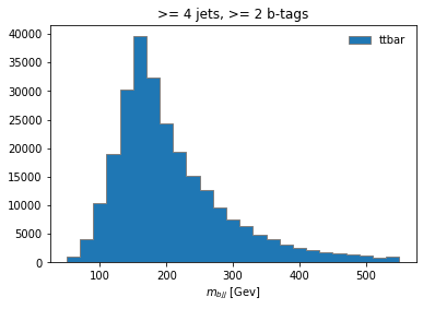
Histogramming and plotting
More information on this topic, including a very instructive video, can be found in one of the tutorials of the IRIS-HEP AGC Tools 2021 Workshop. We will not go into the details here, but just show you some examples.
We will use Hist from the hist package.
So, now we have a flat array for our observable. What else do we need for plotting? Well, a histogram is essentially a way to reduce our data. We can’t just plot every value of trijet mass, so we divide up our range of masses into n bins across some reasonable range. Thus, we need to define the mapping for our reduction; defining the number of bins and the range is sufficient for this. This is called a Regular axis in the hist.Hist package.
In our case, let’s plot 25 bins between values of 50 and 550. Because a histogram can contain an arbitrary amount of axes, we also need to give our axis a name (which becomes its reference in our code) and a label (which is the label on the axis that users see when the histogram is plotted).
Since we will be using several datasets (for signal, background and collisions data) we need a way of keeping these contributions separate in our histograms. One can do with this using Categorical axes. A Categorical axis takes a name, a label, and a pre-defined list of categories. Let’s book a generic histogram with such capabilities:
# This defines the histogram object, but doesn't actually fill it with the data.

histogram = hist.Hist.new.Reg(25, 50, 550,
                              name="observable", label="observable [GeV]")\
                             .StrCat(["4j1b", "4j2b"], name="region", label="Region")\
                             .StrCat([], name="process", label="Process", growth=True)\
                             .StrCat([], name="variation", label="Systematic variation", growth=True)\
                             .Weight()
This histogram placeholder is of type that can accep a Weight to the data tha goes in. This is because for simulated MC samples (backgrounds)
, we will need to normalize the number of events to the total integrated luminosity.
By the way, if you look at the documentation,
help(hist.Hist.new)
you will find
|  Reg = Regular(self, bins: 'int', start: 'float', stop: 'float', *, name: 'str' = '', label: 'str' = '', metadata: 'Any' = None, flow: 'bool' = True, underflow: 'bool | None' = None, overflow: 'bool | None'
= None, growth: 'bool' = False, circular: 'bool' = False, transform: 'AxisTransform | None' = None, __dict__: 'dict[str, Any] | None' = None) -> 'ConstructProxy'
 |
 |  Regular(self, bins: 'int', start: 'float', stop: 'float', *, name: 'str' = '', label: 'str' = '', metadata: 'Any' = None, flow: 'bool' = True, underflow: 'bool | None' = None, overflow: 'bool | None' = None
, growth: 'bool' = False, circular: 'bool' = False, transform: 'AxisTransform | None' = None, __dict__: 'dict[str, Any] | None' = None) -> 'ConstructProxy'
It is useful at this point to do:
print(histogram.ndim)
print()

print(histogram.axes)
in order to understand the structure a bit better. You can see that this hist object is multidimensional holder for histograms, which makes it very convenient and very powerful. You could fill out the outter most StrCategories with several processes and variations. You can slice and dice. Here a very quick example: let’s say that, once the histogram is filled (we haven’t done that yet), you want to get the histograms which have to with the signal region. Accessing them is very simple:
histogram[:,1,:,:]
Now, let’s fill in the histogram:
histogram.fill(observable=observable, region="4j2b", process="ttbar", variation="nominal", weight=1)
and then plot
histogram[:,"4j2b","ttbar","nominal"].plot(histtype="fill", linewidth=1, edgecolor="grey", label='ttbar')
plt.legend()
plt.title(">= 4 jets, >= 2 b-tags")
plt.xlabel("$m_{bjj}$ [Gev]");
plt.show()
Coffea Processors
We now see how simple it could be to construct an analysis using python tools. Naturally, we would like to scale it up to a far larger datasets in any practical scenario. So the first expansion we can do to our analysis is to consider running it over more datasets, which include all of our data, our background, and the signal. Additionally, we would like to show to how to *estimate a few sources of systematic uncertainty, and for that we will be using, in some cases, additional datasets. These systematics datasets are generaly variations of the nominal ones.
To expand our analysis, we will use coffea Processors. Processors are coffea’s way of encapsulating an analysis in a way that is deployment-neutral. Once you have a Coffea analysis, you can throw it into a processor and use any of a variety of executors (e.g. Dask, Parsl, Spark) to chunk it up and run it across distributed workers. This makes scale-out simple and dynamic for users. Unfortunately, we don’t have the time to do such a demostration, but we will run it locally, with our vanilla coffea executor.
Key Point
If you ever get to use executors that can parallelize across distributed workers (e.g., Dask, Parsl, Spark), note that we can do this in HEP. Events are independent of each other, so if we split our work up and ship it off to different workers, we aren’t violating the data’s integrity. Furthermore, since the output we seek is a histogram, our output is also independent of how the work is split up. As long as each worker maps its data to a histogram, the summation of those histograms will be identical to a single worker processing all of the data. In coffea, an object that behaves in this way is called an accumulator.
Defining our coffea Processor
The processor includes a lot of the physics analysis details:
- event filtering and the calculation of observables,
- event weighting,
- calculating systematic uncertainties at the event and object level,
- filling all the information into histograms that get aggregated and ultimately returned to us by coffea
In the coffeaAnalysis_ttbarljets.py in your copy of the repository you will find the definition of our Processor. It is built as a python class, which nicely encapsulates it and, as advertised, becomes independent of the executor.
Inspect it briefly, you will recognize the basic ingredients that we already explored. The only difference is that it has been modified so it allows for additional features like running over different processes and/or variations of them and filling in corresponding histograms.
Take a look at the Processor implementation
Open the Processor
#------------------------------------
class TtbarAnalysis(processor_base):
#------------------------------------
    #--------------------
    def __init__(self):
    #--------------------
        num_bins = 25
        bin_low = 50
        bin_high = 550
        name = "observable"
        label = "observable [GeV]"
        #https://hist.readthedocs.io/en/latest/user-guide/quickstart.html
        #StrCat = StrCategory
        #https://hist.readthedocs.io/en/latest/banner_slides.html?highlight=StrCategory#many-axis-types
        self.hist = (
            hist.Hist.new.Reg(num_bins, bin_low, bin_high, name=name, label=label)
            .StrCat(["4j1b", "4j2b"], name="region", label="Region")
            .StrCat([], name="process", label="Process", growth=True)
            .StrCat([], name="variation", label="Systematic variation", growth=True)
            .Weight()
        )
    #-------------------------
    def process(self, events):
    #-------------------------
        histogram = self.hist.copy()

        process = events.metadata["process"]  # "ttbar" etc.
        variation = events.metadata["variation"]  # "nominal", "scaledown", etc.

        #print(f'Currently doing variation {variation} for {process}')

        # normalization for MC
        x_sec = events.metadata["xsec"]
        nevts_total = events.metadata["nevts"]
        # This truelumi number was obtained with
# brilcalc lumi -c web -i Cert_13TeV_16Dec2015ReReco_Collisions15_25ns_JSON_v2.txt -u /pb --normtag normtag_PHYSICS_2015.json  --begin 256630 --end 260627 > lumi2015D.txt
        # lumi in units of /pb
        lumi = 2256.38
        if process != "data":
            xsec_weight = x_sec * lumi / nevts_total
        else:
            xsec_weight = 1

        #### systematics
        # example of a simple flat weight variation, using the coffea nanoevents systematics feature
        # https://github.com/CoffeaTeam/coffea/blob/20a7e749eea3b8de4880088d2f0e43f6ef9d7993/coffea/nanoevents/methods/base.py#L84
        # Help on method add_systematic in module coffea.nanoevents.methods.base:
        # add_systematic(name: str, kind: str, what: Union[str, List[str], Tuple[str]], varying_function: Callable)
        # method of coffea.nanoevents.methods.base.NanoEventsArray instance
        if process == "wjets":
            events.add_systematic("scale_var", "UpDownSystematic", "weight", flat_variation)

        # example on how to get jet energy scale / resolution systematics
        # need to adjust schema to instead use coffea add_systematic feature, especially for ServiceX
        # cannot attach pT variations to events.jet, so attach to events directly
        # and subsequently scale pT by these scale factors
        events["pt_nominal"] = 1.0
        #events["pt_scale_up"] = 1.03
        # we have already these corrections in our data for this workshop, so we might as well use them
        # to assign a variation per jet and not per event. However, to avoid messing too much with this code,
        # try a silly thing just for fun: take the average of jet variations per event (fill out the None values with a default 1.03)
        events['pt_scale_up'] = ak.fill_none(ak.mean(events.jet.corrptUp/events.jet.corrpt,axis=1),1.03)
        events["pt_res_up"] = jet_pt_resolution(events.jet.corrpt)

        pt_variations = ["pt_nominal", "pt_scale_up", "pt_res_up"] if variation == "nominal" else ["pt_nominal"]
        for pt_var in pt_variations:

            ### event selection
            # based on https://link.springer.com/article/10.1007/JHEP09(2017)051

            #object filters
            > > selected_electrons = events.electron[(events.electron.pt > 30) & (abs(events.electron.eta)<2.1) & (events.electron.isTight == True) & (events.electron.sip3d < 4)]
            > > selected_muons = events.muon[(events.muon.pt > 30) & (abs(events.muon.eta)<2.1) & (events.muon.isTight == True) & (events.muon.sip3d < 4) & (events.muon.pfreliso04DBCorr < 0.15)]
            jet_filter = (events.jet.corrpt * events[pt_var] > 30) & (abs(events.jet.eta)<2.4)
            selected_jets = events.jet[jet_filter]

            # single lepton requirement
            event_filters = ((ak.count(selected_electrons.pt, axis=1) + ak.count(selected_muons.pt, axis=1)) == 1)
            # at least four jets
            pt_var_modifier = events[pt_var] if "res" not in pt_var else events[pt_var][jet_filter]
            event_filters = event_filters & (ak.count(selected_jets.corrpt * pt_var_modifier, axis=1) >= 4)
            # at least one b-tagged jet ("tag" means score above threshold)
            B_TAG_THRESHOLD = 0.8
            event_filters = event_filters & (ak.sum(selected_jets.btag >= B_TAG_THRESHOLD, axis=1) >= 1)

            # apply event filters
            selected_events = events[event_filters]
            selected_electrons = selected_electrons[event_filters]
            selected_muons = selected_muons[event_filters]
            selected_jets = selected_jets[event_filters]

            for region in ["4j1b", "4j2b"]:
                # further filtering: 4j1b CR with single b-tag, 4j2b SR with two or more tags
                if region == "4j1b":
                    region_filter = ak.sum(selected_jets.btag >= B_TAG_THRESHOLD, axis=1) == 1
                    selected_jets_region = selected_jets[region_filter]
                    # use HT (scalar sum of jet pT) as observable
                    pt_var_modifier = events[event_filters][region_filter][pt_var] if "res" not in pt_var else events[pt_var][jet_filter][event_filters][region_filter]
                    observable = ak.sum(selected_jets_region.corrpt * pt_var_modifier, axis=-1)

                elif region == "4j2b":
                    region_filter = ak.sum(selected_jets.btag > B_TAG_THRESHOLD, axis=1) >= 2
                    selected_jets_region = selected_jets[region_filter]

                    # reconstruct hadronic top as bjj system with largest pT
                    # the jet energy scale / resolution effect is not propagated to this observable at the moment
                    trijet = ak.combinations(selected_jets_region, 3, fields=["j1", "j2", "j3"])  # trijet candidates
                    trijet["p4"] = trijet.j1 + trijet.j2 + trijet.j3  # calculate four-momentum of tri-jet system
                    trijet["max_btag"] = np.maximum(trijet.j1.btag, np.maximum(trijet.j2.btag, trijet.j3.btag))
                    trijet = trijet[trijet.max_btag > B_TAG_THRESHOLD]  # require at least one-btag in trijet candidates
                    # pick trijet candidate with largest pT and calculate mass of system
                    trijet_mass = trijet["p4"][ak.argmax(trijet.p4.pt, axis=1, keepdims=True)].mass
                    observable = ak.flatten(trijet_mass)

                ### histogram filling
                if pt_var == "pt_nominal":
                    # nominal pT, but including 2-point systematics
                    histogram.fill(
                            observable=observable, region=region, process=process, variation=variation, weight=xsec_weight
                        )


                    if variation == "nominal":
                        # also fill weight-based variations for all nominal samples
                        # this corresponds to the case for wjets included above as an example
                        for weight_name in events.systematics.fields:
                            for direction in ["up", "down"]:
                                # extract the weight variations and apply all event & region filters
                                weight_variation = events.systematics[weight_name][direction][f"weight_{weight_name}"][event_filters][region_filter]
                                # fill histograms
                                histogram.fill(
                                    observable=observable, region=region, process=process, variation=f"{weight_name}_{direction}", weight=xsec_weight*weight_variation
                                )

                        # calculate additional systematics: b-tagging variations
                        for i_var, weight_name in enumerate([f"btag_var_{i}" for i in range(4)]):
                            for i_dir, direction in enumerate(["up", "down"]):
                                # create systematic variations that depend on object properties (here: jet pT)
                                if len(observable):
                                    weight_variation = btag_weight_variation(i_var, selected_jets_region.corrpt)[:, i_dir]
                                else:
                                    weight_variation = 1 # no events selected
                                histogram.fill(
                                    observable=observable, region=region, process=process, variation=f"{weight_name}_{direction}", weight=xsec_weight*weight_variation
                                )

                elif variation == "nominal":
                    # pT variations for nominal samples
                    histogram.fill(
                            observable=observable, region=region, process=process, variation=pt_var, weight=xsec_weight
                        )
        output = {"nevents": {events.metadata["dataset"]: len(events)}, "hist": histogram}

        return output
    # https://coffeateam.github.io/coffea/api/coffea.processor.ProcessorABC.html?highlight=postprocess#coffea.processor.ProcessorABC.postprocess
    def postprocess(self, accumulator):
        return accumulator
Right below this Processor class, in the coffeaAnalysis_ttbarljets.py file, you will find a snippet which builds the input for the Processor (i.e., for the analysis):
# "Fileset" construction and metadata via utils.py file
# Here, we gather all the required information about the files we want to process: paths to the files and asociated metadata
# making use of the utils.py code in this repository
fileset = construct_fileset(N_FILES_MAX_PER_SAMPLE, use_xcache=False)
print(f"processes in fileset: {list(fileset.keys())}")
print(f"\nexample of information in fileset:\n { {\n  'files': [{fileset['ttbar__nominal']['files'][0]}, ...],")
print(f"  'metadata': {fileset['ttbar__nominal']['metadata']}\n } }")
t0 = time.time()
This is done with the help of the function construct_fileset, which is part of the utils.py file that you can also find in the repository. After you import the code in this file (like it is done in the heade of coffeaAnalysis_ttbarljets.py),
# Slimmed version of:
# https://github.com/iris-hep/analysis-grand-challenge/tree/main/analyses/cms-open-data-ttbar/utils
# These file contain code for bookkeeping and cosmetics, as well as some boilerplate
from utils import *
you get some utilities like styling routines and the fileset builder. Note that it is here where the cross sections for the different samples are stored. Also, the ntuples.json file (also find it in the repository) is read here to manage the fileset that will be fed to the Processor. We do some gymnastics also to adjust the normalization correctly. Finally there is a function to save the histograms in a ROOT file.
Next, in the coffeaAnalysis_ttbarljets.py file, you will see the call-out for the executor:
#Execute the data delivery pipeline
#we don't have an external executor, so we use local coffea (IterativeExecutor())
if PIPELINE == "coffea":
    executor = processor.IterativeExecutor()
    from coffea.nanoevents.schemas.schema import auto_schema
    schema = AGCSchema if PIPELINE == "coffea" else auto_schema
    run = processor.Runner(executor=executor, schema=schema, savemetrics=True, metadata_cache={})
    all_histograms, metrics = run(fileset, "events", processor_instance=TtbarAnalysis())
    all_histograms = all_histograms["hist"]
It is here where you decide where to run. Unfortunately, the datasets over which we are running are still quite large. So running on the whole dataset in a single computer is not very efficient. It will take a long time. Here is where coffea really performs, because you can ship it to different worker nodes using some different executors.
Finally note that there are some auxiliary functions at the beginning of the coffeaAnalysis_ttbarljets.py file and some histogramming routines at the end. We won’t worry about them for now.
Stop Jupyter Lab
We’re going to run a couple of commands now from the shell environment by calling some python scripts. So first, we need to save our work and shutdown Jupyter Lab.
Before saving our work, let’s stop the kernel and clear the output. That way we won’t save all the data and the notebook.
Click on Kernel and then Restart Kernel and Clear All Outputs.
Then, click on File and then Save Notebook.
Then, click on File and then Shut Down. You should now have your prompt back in the terminal with your Docker instance!
Running an example of the analysis
If you have a good connection you may get to run over just a single file per dataset by setting the N_FILES_MAX_PER_SAMPLE = 1 at the beggining of the coffeaAnalysis_ttbarljets.py file. Otherwise, do not worry we will provide you with the final histograms.root output after we ran over the whole dataset (for reference, it takes about 4 hours in a regular laptop).
If you have time! (probably not right now)
Edit
coffeaAnalysis_ttbarljets.pyso thatN_FILES_MAX_PER_SAMPLE = 1rather thanN_FILES_MAX_PER_SAMPLE = -1. And then run the demonstrator:cd /code/workshop2022-lesson-ttbarljetsanalysis-payload python coffeaAnalysis_ttbarljets.pyThis can take quite some time, even running over 1 file in each dataset, so you may want to do this on your own time and not during the synchronous parts of this workshop.
Plotting
Plotting the final results
Here you can download a full
histograms.root. It was obtained after 4 hours of running on a single computer. When you click on the link, you’ll be directed to CERNBox, a tool to share large files, similar to DropBox.To download the file, click on the three (3) vertical dots by the
histograms.rootname in the tab near the top. Then select Download.When the file is downloaded, move it to to your
cms_open_data_python/workshop2022-lesson-ttbarljetsanalysis-payloadon your local laptop. Because this directory is mounted in your Docker container, you will be able to see this file in Docker.Of course, if you have some available space, you could download the files (the size is not terribly large, maybe around 60GB or so), and run much faster. It contains all the histograms produced by the analysis Processor. We have prepared a plotting script for you to see the results:
python plotme.py
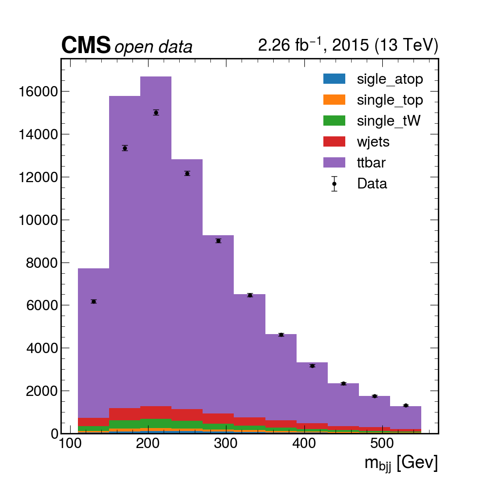
Pretty good! The data mostly seems to match up with our assumptions about how much the different MC samples contribute, but maybe we can do better if we allow for the fact that we may not know these values exactly. In the next section, we’ll try to use some inference tools to get a more precise description of the data!
Key Points
Basic selection requirements are implemented very easily using columnar analysis
Coffea processors encapsulate an analysis so it becomes deployment-neutral
Break
Overview
Teaching: 0 min
Exercises: 30 minQuestions
Should we get some coffea?
Objectives
Get some coffea and some refreshments
Break well-deserved, we will see you again in 30’.
Key Points
We will definitely get some coffea
Systematics and Statistics
Overview
Teaching: 90 min
Exercises: 0 minQuestions
How are systematic variations handled in Coffea?
How do we perform statistical inference?
What tools do we use?
How do we visualize and interpret our results?
Objectives
Explore some examples for adding systematic variations in Coffea
Learn how to construct statistical models.
Learn how to interpret these statistical models.
Systematics in Coffea
In an analysis such as this one there are many systematics to consider, both experimental and theoretical (as encapsulated in the MC). For the former these include trigger and selection efficiencies, jet energy scale and resolution, b-tagging and misidentification efficiencies, and integrated luminosity. The latter can include uncertainties due to choice of hadronizer, choice of generator, QCD scale choices, and the parton shower scale. This isn’t a complete list of systematics and here we will only cover a few of these.
Let’s explore the different ways in which one can introduce the estimation of systematic uncertainties in Coffea. A few examples, which are relevant for our analysis, have been implemented by the original \(t\bar{t}\) AGC demonstration. Of course, they are part of our coffeaAnalysis_ttbarljets.py code. Let’s explore the different pieces:
Before, we begin, note that a multidimensional array for histograms has been booked:
    #--------------------
    def __init__(self):
    #--------------------
        num_bins = 25
        bin_low = 50
        bin_high = 550
        name = "observable"
        label = "observable [GeV]"
        #https://hist.readthedocs.io/en/latest/user-guide/quickstart.html
        #StrCat = StrCategory
        #https://hist.readthedocs.io/en/latest/banner_slides.html?highlight=StrCategory#many-axis-types
        self.hist = (
            hist.Hist.new.Reg(num_bins, bin_low, bin_high, name=name, label=label)
            .StrCat(["4j1b", "4j2b"], name="region", label="Region")
            .StrCat([], name="process", label="Process", growth=True)
            .StrCat([], name="variation", label="Systematic variation", growth=True)
            .Weight()
        )
The different processes (associated with our main datasets for data, signal and backgrounds) and variations (also datasets but variations of the nominal one) are passed to the Processor:
    #-------------------------
    def process(self, events):
    #-------------------------
        histogram = self.hist.copy()

        process = events.metadata["process"]  # "ttbar" etc.
        variation = events.metadata["variation"]  # "nominal", "scaledown", etc.

        #print(f'Currently doing variation {variation} for {process}')
Monte Carlo simulations are normalized to the actual luminosity. Cross sections and numbers of total events for the different samples are also passed to the Processor. They are handled by the utils.py program, as you may remember:
        # normalization for MC
        x_sec = events.metadata["xsec"]
        nevts_total = events.metadata["nevts"]
        # This lumi number was obtained with
        # brilcalc lumi -c web -i Cert_13TeV_16Dec2015ReReco_Collisions15_25ns_JSON_v2.txt -u /pb --normtag normtag_PHYSICS_2015.json  --begin 256630 --end 260627 > lumi2015D.txt
        # lumi in units of /pb
        lumi = 2256.38
        if process != "data":
            xsec_weight = x_sec * lumi / nevts_total
        else:
            xsec_weight = 1
There are several ways in which one can introduce systematic variations. A built-in option provided by Coffea, add_systematics, is the easiest. Here an example of a made up variation for the scale of the wjets contribution:
        #### systematics
        # example of a simple flat weight variation, using the coffea nanoevents systematics feature
        # https://github.com/CoffeaTeam/coffea/blob/20a7e749eea3b8de4880088d2f0e43f6ef9d7993/coffea/nanoevents/methods/base.py#L84
        # Help on method add_systematic in module coffea.nanoevents.methods.base:
        # add_systematic(name: str, kind: str, what: Union[str, List[str], Tuple[str]], varying_function: Callable)
        # method of coffea.nanoevents.methods.base.NanoEventsArray instance
        if process == "wjets":
            events.add_systematic("scale_var", "UpDownSystematic", "weight", flat_variation)
We do have per-jet variations in our ntuples now, but by the time this AGC demonstrator was written we did not. This is an example of how to add variatinos for jet energy scale and resolution with a per-event number. To make use of the information we have without varying the code too much, we test a silly average for the jet energy scale:
        # example on how to get jet energy scale / resolution systematics
        # need to adjust schema to instead use coffea add_systematic feature, especially for ServiceX
        # cannot attach pT variations to events.jet, so attach to events directly
        # and subsequently scale pT by these scale factors
        events["pt_nominal"] = 1.0
        #events["pt_scale_up"] = 1.03
        # we have already these corrections in our data for this workshop, so we might as well use them
        # to assign a variation per jet and not per event. However, to avoid messing too much with this code,
        # try a silly thing just for fun: take the average of jet variations per event (fill out the None values with a default 1.03)
        events['pt_scale_up'] = ak.fill_none(ak.mean(events.jet.corrptUp/events.jet.corrpt,axis=1),1.03)
        events["pt_res_up"] = jet_pt_resolution(events.jet.corrpt)

        pt_variations = ["pt_nominal", "pt_scale_up", "pt_res_up"] if variation == "nominal" else ["pt_nominal"]
The routine then loops over these different types of variations also separating the two signal and control regions, performing the same basic analysis we defined before:
for pt_var in pt_variations:
    ...
    for region in ["4j1b", "4j2b"]:
For the nominal samples, it is this snippet which introduces the scale variation which might have been included earlier (this is the case for the wjets above):
if variation == "nominal":
                        # also fill weight-based variations for all nominal samples
                        # this corresponds to the case for wjets included above as an example
                        for weight_name in events.systematics.fields:
                            for direction in ["up", "down"]:
                                # extract the weight variations and apply all event & region filters
                                weight_variation = events.systematics[weight_name][direction][f"weight_{weight_name}"][event_filters][region_filter]
                                # fill histograms
                                histogram.fill(
                                    observable=observable, region=region, process=process, variation=f"{weight_name}_{direction}", weight=xsec_weight*weight_variation
                                )
Finally an example of how to generate variations that may depend on objects properties, like jet \(p_{T}\) for the b-tagging. Note that we already have these variations included in our ntuples but chose not to use them to preserve this version of the demonstration:
# calculate additional systematics: b-tagging variations
                        for i_var, weight_name in enumerate([f"btag_var_{i}" for i in range(4)]):
                            for i_dir, direction in enumerate(["up", "down"]):
                                # create systematic variations that depend on object properties (here: jet pT)
                                if len(observable):
                                    weight_variation = btag_weight_variation(i_var, selected_jets_region.corrpt)[:, i_dir]
                                else:
                                    weight_variation = 1 # no events selected
                                histogram.fill(
                                    observable=observable, region=region, process=process, variation=f"{weight_name}_{direction}", weight=xsec_weight*weight_variation
                                )
Introduction to stats analysis
It’s beyond the scope of this tutorial to cover a lot of statistical background needed here. You may find some references at the end of this episode and further references found within. We will cover hopefully the bare-minimum needed to give you an idea of what’s going on here and to give an introduction to some useful tools.
A statistical model \(f(\vec{x} \vert \vec{\phi})\) describes the probability of the data \(\vec{x}\) given model paramters \(\vec{\phi}\).
HistFactory is a tool to construct probabilty distribution functions from template histograms, constructing a likelihood function. In this exercise we will be using HistFactory via pyhf, a python implementation of this tool. In addition, we will be using the cabinetry package, which is a python library for constructing and implementing HistFactory models.
The HistFactory template model can expressed like this:

What’s here?
- \(\vec{n}\) describes the observed channel data and \(\vec{a}\) describes the auxiliary data e.g. from calibration
- \(\vec{\eta}\) describes the unconstrained parameters (parameters of interest POI) and \(\vec{\chi}\) the constrained parameters (nuisance parameters NPs)
- \(n_{cb}\): the observed number of events, \(\nu_{nb}(\vec{\eta}, \vec{\chi})\): expected number of events
- Main poisson p.d.f. for simultaneous measurement over multiple channels (or regions, like a signal region and a control region) and bins (over the histograms)
- Constraint p.d.f which encodes systematic uncertainties: the actual function used depends on the parameter (e.g. it may be a Gaussian)
- Parameters of interest (POIs): examples in analyses include \(\sigma \times B\), \(m_{W}\), …
- Nuisance parameters (NPs): other parameters needed to define the model, e.g. luminosity
This is a lot to take in but we’ll press on regardless with implementation.
Essentially:
HistFactoryis a model used for binned statistical analysispyhfis a python implementation of this modelcabinetrycreates a statistical model from a specification of cuts, systematics, samples, etc.pyhfthen turns this model into a likelihood function
Making models and fitting
It should be noted that everything in this part is contained in the
use_cabinetry.pyscript. This file can be found in your copy of the lesson repository
Histograms
Let’s quickly inspect our histograms in the histograms.root file by running ROOT and opening
up a TBrowser.
Try this if you have ROOT installed and have gone through the ROOT pre-exercise. If not, skip this part and try it later. We’ll show the output below anyway.
root histograms.root
   ------------------------------------------------------------------
  | Welcome to ROOT 6.26/00                        https://root.cern |
  | (c) 1995-2021, The ROOT Team; conception: R. Brun, F. Rademakers |
  | Built for linuxx8664gcc on Jun 14 2022, 14:46:00                 |
  | From tag , 3 March 2022                                          |
  | With c++ (Ubuntu 9.4.0-1ubuntu1~20.04.1) 9.4.0                   |
  | Try '.help', '.demo', '.license', '.credits', '.quit'/'.q'       |
   ------------------------------------------------------------------

root [0]
Attaching file histograms.root as _file0...
(TFile *) 0x563baef326f0
root [1] TBrowser b
(TBrowser &) Name: Browser Title: ROOT Object Browser
Click on one of the histogram titles on the left for 4j1b to view it:

Click on another for 4j2b:

Recall that our observable for the 4j1b control region is the scalar sum of jet transverse momentum, \(H_{T}\) and our observable for the 4j2b signal region is the mass of b-jet system \(m_{b_{jj}}\).
Start up a Jupyter notebook
Follow the steps from the previous episode to fire up Jupyter Lab, create a Jupyter notebook,
and name it ttbar_inference.ipynb.
Let’s start by importing the necessary modules (if you haven’t already), most importantly cabinetry:
import logging
import cabinetry
If cabinetry is not installed:
pip install cabinetry
Cabinetry workspace
A statistical model can be define in a declarative way using cabinetry, capturing the \(\mathrm{region \otimes sample \otimes systematic}\) structure.
General settings General:, list of phase space regions such as signal and control regions Regions:, list of samples (MC and data) Samples:, list of systematic uncertainties Systematics:, and a list of normalization factors NormFactors:.
Let’s have a look at each of the parts of the the configuration file, workshop2022-lesson-ttbarljetsanalysis-payload$/cabinetry_config.yml:
General
General:
  Measurement: "CMS_ttbar"
  POI: "ttbar_norm"
  HistogramFolder: "histograms/"
  InputPath: "histograms.root:{RegionPath}_{SamplePath}{VariationPath}"
  VariationPath: ""
Regions
Regions:
  - Name: "4j1b CR"
    RegionPath: "4j1b"

  - Name: "4j2b SR"
    RegionPath: "4j2b"
Samples
Samples:
  - Name: "Pseudodata"
    SamplePath: "pseudodata"
    Data: True

  - Name: "ttbar"
    SamplePath: "ttbar"

  - Name: "W+jets"
    SamplePath: "wjets"

  - Name: "single top, t-channel"
    SamplePath: "single_top_t_chan"

  - Name: "single atop, t-channel"
    SamplePath: "single_atop_t_chan"

  - Name: "tW"
    SamplePath: "single_top_tW"
Systematics
Systematics:
  - Name: "ME variation"
    Type: "NormPlusShape"
    Up:
      VariationPath: "_ME_var"
    Down:
      Symmetrize: True
    Samples: "ttbar"

  - Name: "PS variation"
    Type: "NormPlusShape"
    Up:
      VariationPath: "_PS_var"
    Down:
      Symmetrize: True
    Samples: "ttbar"
Here we specify which systematics we want to take into account. In addition to the W+jets scale variations, b-tagging variations, and jet energy scale and resolution (shown in the full file) we show here for the ttbar samples _ME_var (what do the result look like if we choose another generator?) and _PS_var (what do the results look like if we use a different hadronizer?).
NormFactors
NormFactors:
  - Name: "ttbar_norm"
    Samples: "ttbar"
    Nominal: 1.0
    Bounds: [0, 10]
Running cabinetry and results
Let’s load the cabinetry configuration file and combine the histograms into a pyhf workspace which we will save:
config = cabinetry.configuration.load("cabinetry_config.yml")

cabinetry.templates.collect(config)

ws = cabinetry.workspace.build(config)

cabinetry.workspace.save(ws, "workspace.json")
You may see a number of warnings, but you can ignore them.
pyhf can be run on the command line to inspect the workspace:
pyhf inspect workspace
Or you can run it inside of your Jupyter notebook by typing
!pyhf inspect workspace.json
where the ! exclamation point tells Jupyter to run the command as a bash command and return the output.
Either of these commands outputs the following:
                 Summary
            ------------------
               channels  2
                samples  5
             parameters  14
              modifiers  14

               channels  nbins
             ----------  -----
                4j1b CR   11
                4j2b SR   11

                samples
             ----------
                 W+jets
 single atop, t-channel
  single top, t-channel
                     tW
                  ttbar

            parameters  constraint              modifiers
             ----------  ----------              ----------
  Jet energy resolution  constrained_by_normal   histosys,normsys
       Jet energy scale  constrained_by_normal   histosys,normsys
             Luminosity  constrained_by_normal   normsys
           ME variation  constrained_by_normal   histosys,normsys
           PS variation  constrained_by_normal   histosys,normsys
W+jets scale variations  constrained_by_normal   histosys,normsys
             b-tag NP 1  constrained_by_normal   histosys,normsys
             b-tag NP 2  constrained_by_normal   histosys,normsys
             b-tag NP 3  constrained_by_normal   histosys,normsys
             b-tag NP 4  constrained_by_normal   histosys,normsys
      staterror_4j1b-CR  constrained_by_normal   staterror
      staterror_4j2b-SR  constrained_by_normal   staterror
 ttbar scale variations  constrained_by_normal   histosys,normsys
             ttbar_norm  unconstrained           normfactor

            measurement           poi            parameters
             ----------        ----------        ----------
          (*) CMS_ttbar        ttbar_norm        ttbar_norm
Now we perform our maximum likelihood fit
model, data = cabinetry.model_utils.model_and_data(ws)

fit_results = cabinetry.fit.fit(model, data)
and visualize the pulls of parameters in the fit:
pull_fig = cabinetry.visualize.pulls(
    fit_results, exclude="ttbar_norm", close_figure=True, save_figure=True
)

pull_fig

Your plot might look different as the order of the systematics might be different, though the values should be the same.
What are pulls? For our nuisance parameters in the fit the pull is defined as \((\hat{\theta} - \theta_{0}) / \Delta\theta\), which is the difference between the fitted parameter value and the initial value divided by the width. Looking at the pulls can aid in seeing how well (or how badly) your fit performed. For unbiased estimates and correctly estimated uncertainties, the pull should have a central value of 0 and an uncertainty of 1. If the central value is not 0 then some data feature differs from the expectation which may need investigation if large. If the uncertainty is less than 1 then something is constrained by the data. This needs checking to see if this is legitimate or a modeling issue.
Note that the figures produced by running the script or your commands are to be found in the
figures/ directory.
What does the model look like before and after the fit? We can visualize each with the following code:
# Before the fit

model_prediction = cabinetry.model_utils.prediction(model)

figs = cabinetry.visualize.data_mc(model_prediction, data, close_figure=False)
# After the fit

model_prediction_postfit = cabinetry.model_utils.prediction(model, fit_results=fit_results)

figs = cabinetry.visualize.data_mc(model_prediction_postfit, data, close_figure=False)
We can see that there is very good post-fit agreement:
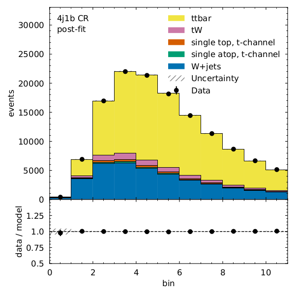
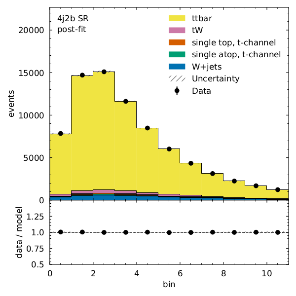
Finally, what’s the \(t\bar{t}\) cross section (for our pseudodata) divided by the Standard Model prediction?
poi_index = model.config.poi_index

print(f"\nfit result for ttbar_norm: {fit_results.bestfit[poi_index]:.3f} +/- {fit_results.uncertainty[poi_index]:.3f}")
fit result for ttbar_norm: 0.964 +/- 0.075
Phew. We covered a lot in a very short time but essentially:
- Coffea allows for addition of systematic variations
- Our likelihood structure allows us to include systematics as uncertainties on NPs
- The statistical model uses the HistFactory template
- This is implemented using
pyhfandcabinetryWhat wasn’t covered? A lot. But hopefully there is enough here to get you started.
References and further reading
Acknowledgements
Thanks to the authors of the AGC using CMS data on which much of the episode was based.
Key Points
Systematic variations are conveniently handled with Coffea
We construct statistical models to estimate systematics in our analysis.
cabinetryandpyhfare the tools we use here.