Introduction
Overview
Teaching: 20 min
Exercises: 20 minQuestions
What analysis will we be doing?
What is columnar analysis?
Why do we use coffea?
What are coffea main components?
What are schemas?
Objectives
Learn about the physics behind the analysis example.
Learn about the strategy we will follow for our analysis example.
Learn what the difference is between columnar and loop analysis.
Learn what coffea is and what the logic is of its different compoonets
Learn about what schemas are used for and how to modify them
Physics introduction
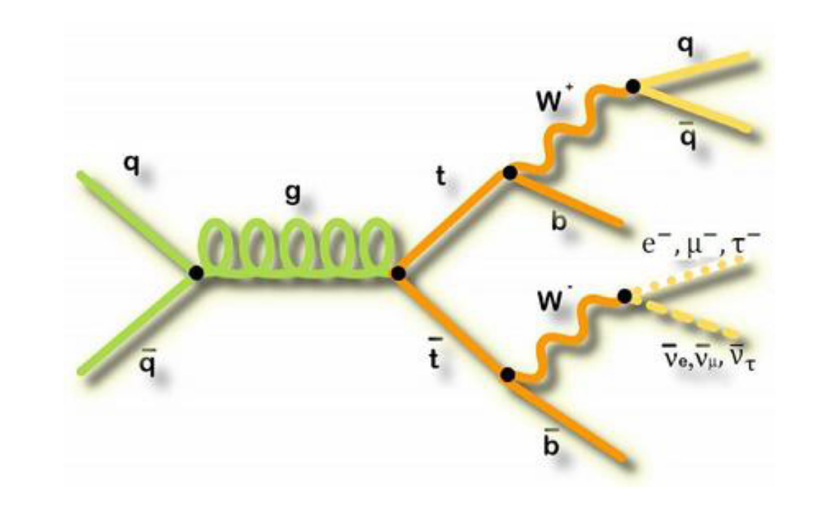
In this lesson, you will be walked through a mini-reproduction of a 2017 analysis from the CMS collaboration. The cross-section for the production of top-quark / anti-top-quark pairs in proton-proton collisions was measured. Put another way, we measured the probability that a top-quark and an anti-top quark pair are produced when protons are collided at a center-of-mass energy of 13 TeV.
 .
.
To go into a bit more detail
in this simplified analysis we will be working towards a measurement of the top and anti-top quark production cross section \(\sigma_{t\bar{t}}\).
The data are produced in proton-proton collisions at \(\sqrt{s}\) = 13 TeV at the beginning of Run 2 of the LHC. We will be examining the lepton+jets final state
\(t\bar{t} \rightarrow (bW^{+})(\bar{b}W_{-}) \rightarrow bq\bar{q} bl^{-}\bar{\nu_{l}}\)
which is characterized by one lepton (here we look at electrons and muons only), significant missing transverse energy, and four jets, two of which are identified as b-jets.
Slides
We want to motivate why we are encouraging you to look into some of these newer software tools. Let’s go through these slides together to review this analysis and to get a more complete overview of what goes into an analysis.
Coding (python) introduction
We will attempt to use tools that are built on modern, powerful and efficient python ecosystems. In particular, we will use the Columnar Object Framework For Effective Analysis (Coffea), which will provide us with basic tools and wrappers for enabling not-too-alien syntax when running columnar Collider HEP analysis.
Start up Docker and JupyterLab
Type out the following commands for this episode!
For this next section, you’ll be asked to type out the provided commands in a Jupyter notebook, a popular development environment that allows you to use python in an interactive way.
Please enter in these commands yourself for this episode.
To create or run these notebooks, we will
- Start the python docker container
- Install some necessary extra module (this only needs to be done once)
- Launch Jupyter Lab, an application that makes it easier to work with Jupyter Notebooks
- Create a new Jupyter Notebook for this episode.
Start Docker If you have already successfully installed and run the Docker example with python tools, then you need only execute the following command.
docker start -i my_python #give the name of your container
If this doesn’t work, return to the python tools Docker container lesson to work through how to start the container.
Install the extra libraries
(If you did this already by following the setup section of this lesson, then you needn’t do this part again.)
In order to use the coffea framework for our analysis, we need to install these additional packages directly in our container. We are adding
cabinetry as well because we will use it later in our last episode. This can take a few minutes to install.
pip install vector hist mplhep coffea cabinetry
Also, download this file, which is our starting schema. Directly in your /code area (or locally in your cms_open_data_python directory) you can simply do:
wget https://raw.githubusercontent.com/cms-opendata-workshop/workshop2022-lesson-ttbarljetsanalysis-payload/master/trunk/agc_schema.py
Launch Jupyter Lab In your docker python container, type the following.
jupyter-lab --ip=0.0.0.0 --no-browser
Launching Jupyter Lab
You should see something like this in your Docker container terminal when you type the above
jupyter-labcommand.
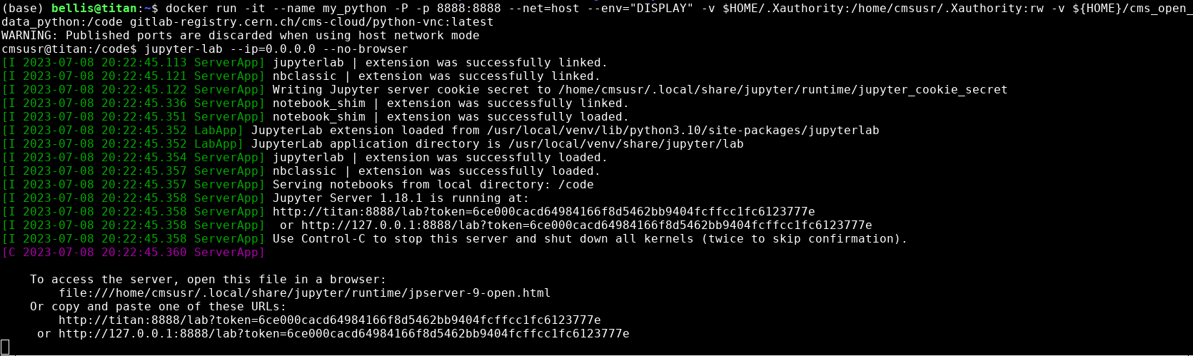
In the image above you can see the output when I start jupyter-lab on my computer. Yours won’t say exactly
the same thing, but it should be similar. Take note of the last two lines that start with http://. Start up a
browser locally on your laptop or desktop (not from the Docker container). Copy one of those
URLs and paste it into the browser. If the first URL doesn’t work, try the other.
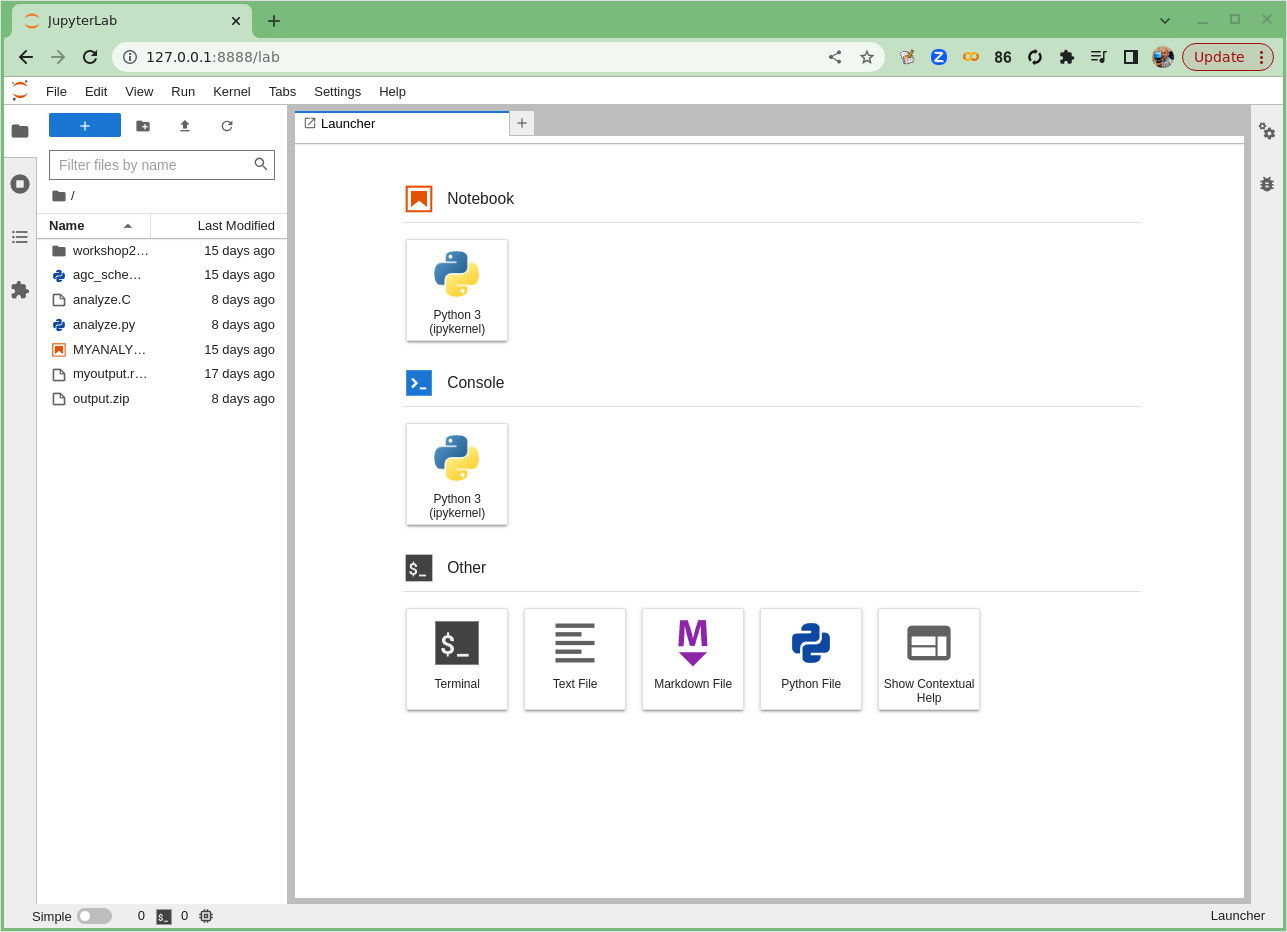
If it works you’ll see something in your browser similar to the following image!
Launching Jupyter Lab
If Jupyter Lab launched, you’ll see something like this.
Start a new Jupyter notebook
The top icon (under Notebook) says Python 3 (ipykernel). Click on this icon. This should launch a new Jupyter notebook!
Starting a new Jupyter notebook
If your new Jupyter Notebook started, you’ll see something like this.

In this Jupyter Lab environment, click on File (in the top right) and then from the dropdown
menu select Rename Notebook…. You can call this notebook whatever you like but I have
called mine analysis_example_prelesson.ipynb.
For the remainder of this lesson, you’ll be typing or cutting-and-pasting the commands you see here in the Python sections into the Jupyter Notebook. To run those commands after you have typed them, you can press the little Play icon (right-pointing triangle) or type Shift + Enter (to run the cell and advance) or Ctrl + Enter (to run the cell and not advance). Whichever you prefer.
Optional! Using ipython
If, for some reason, you don’t want to use Jupyter, you can launch interactive python just by typing
ipythonin Docker Container (and not thejupyter-labcommand) and then entering the python commands there.
Columnar analysis basics with Awkward
Note: this and the next section on this episode are a recast (with some shameless copying and pasting) of this notebook by Mat Adamec presented during the IRIS-HEP AGC Workshop 2022.
In one of the pre-exercises we learned how to access ROOT files (the standard use at the LHC experiments) using uproot and why the awkward library can be very helpufl when dealing with jagged arrays.
Let’s remember very quickly. First, be sure to import the appropriate libraries:
import uproot
import awkward as ak
Let’s open an example file. These are flattened POET ntuples. As it was mentioned in the trigger lesson, we will be producing these skimmed ntuples for you. You may recognize all the variables we had worked with before.
Using uproot,
events = uproot.open('root://eospublic.cern.ch//eos/opendata/cms/upload/od-workshop/ws2021/myoutput_odws2022-ttbaljets-prodv2.0_merged.root')['events']
events
<TTree 'events' (275 branches) at 0x7fb46a8b5870>.
We now have an events tree. We can view its branches by querying its keys():
events.keys()
['numberelectron', 'nelectron_e', 'electron_e', 'nelectron_pt', 'electron_pt', 'nelectron_px', 'electron_px', 'nelectron_py', 'electron_py', 'nelectron_pz', 'electron_pz', 'nelectron_eta', 'electron_eta', 'nelectron_phi', 'electron_phi', 'nelectron_ch', 'electron_ch', 'nelectron_iso', 'electron_iso', 'nelectron_veto', 'electron_veto', 'nelectron_isLoose', 'electron_isLoose', 'nelectron_isMedium', 'electron_isMedium', 'nelectron_isTight', 'electron_isTight', 'nelectron_dxy', 'electron_dxy', 'nelectron_dz', 'electron_dz', 'nelectron_dxyError', 'electron_dxyError', 'nelectron_dzError', 'electron_dzError', 'nelectron_ismvaLoose', 'electron_ismvaLoose', 'nelectron_ismvaTight', 'electron_ismvaTight', 'nelectron_ip3d', 'electron_ip3d', 'nelectron_sip3d', 'electron_sip3d', 'numberfatjet', 'nfatjet_e', 'fatjet_e', 'nfatjet_pt', 'fatjet_pt', 'nfatjet_eta', 'fatjet_eta', 'nfatjet_phi', 'fatjet_phi', 'nfatjet_ch', 'fatjet_ch', 'nfatjet_mass', 'fatjet_mass', 'nfatjet_corrpt', 'fatjet_corrpt', 'nfatjet_corrptUp', 'fatjet_corrptUp', 'nfatjet_corrptDown', 'fatjet_corrptDown', 'nfatjet_corrptSmearUp', 'fatjet_corrptSmearUp', 'nfatjet_corrptSmearDown', 'fatjet_corrptSmearDown', 'nfatjet_corrmass', 'fatjet_corrmass', 'nfatjet_corre', 'fatjet_corre', 'nfatjet_corrpx', 'fatjet_corrpx', 'nfatjet_corrpy', 'fatjet_corrpy', 'nfatjet_corrpz', 'fatjet_corrpz', 'nfatjet_prunedmass', 'fatjet_prunedmass', 'nfatjet_softdropmass', 'fatjet_softdropmass', 'nfatjet_tau1', 'fatjet_tau1', 'nfatjet_tau2', 'fatjet_tau2', 'nfatjet_tau3', 'fatjet_tau3', 'nfatjet_subjet1btag', 'fatjet_subjet1btag', 'nfatjet_subjet2btag', 'fatjet_subjet2btag', 'nfatjet_subjet1hflav', 'fatjet_subjet1hflav', 'nfatjet_subjet2hflav', 'fatjet_subjet2hflav', 'numberjet', 'njet_e', 'jet_e', 'njet_pt', 'jet_pt', 'njet_eta', 'jet_eta', 'njet_phi', 'jet_phi', 'njet_ch', 'jet_ch', 'njet_mass', 'jet_mass', 'njet_btag', 'jet_btag', 'njet_hflav', 'jet_hflav', 'njet_corrpt', 'jet_corrpt', 'njet_corrptUp', 'jet_corrptUp', 'njet_corrptDown', 'jet_corrptDown', 'njet_corrptSmearUp', 'jet_corrptSmearUp', 'njet_corrptSmearDown', 'jet_corrptSmearDown', 'njet_corrmass', 'jet_corrmass', 'njet_corre', 'jet_corre', 'njet_corrpx', 'jet_corrpx', 'njet_corrpy', 'jet_corrpy', 'njet_corrpz', 'jet_corrpz', 'btag_Weight', 'btag_WeightUp', 'btag_WeightDn', 'met_e', 'met_pt', 'met_px', 'met_py', 'met_phi', 'met_significance', 'met_rawpt', 'met_rawphi', 'met_rawe', 'numbermuon', 'nmuon_e', 'muon_e', 'nmuon_pt', 'muon_pt', 'nmuon_px', 'muon_px', 'nmuon_py', 'muon_py', 'nmuon_pz', 'muon_pz', 'nmuon_eta', 'muon_eta', 'nmuon_phi', 'muon_phi', 'nmuon_ch', 'muon_ch', 'nmuon_isLoose', 'muon_isLoose', 'nmuon_isMedium', 'muon_isMedium', 'nmuon_isTight', 'muon_isTight', 'nmuon_isSoft', 'muon_isSoft', 'nmuon_isHighPt', 'muon_isHighPt', 'nmuon_dxy', 'muon_dxy', 'nmuon_dz', 'muon_dz', 'nmuon_dxyError', 'muon_dxyError', 'nmuon_dzError', 'muon_dzError', 'nmuon_pfreliso03all', 'muon_pfreliso03all', 'nmuon_pfreliso04all', 'muon_pfreliso04all', 'nmuon_pfreliso04DBCorr', 'muon_pfreliso04DBCorr', 'nmuon_TkIso03', 'muon_TkIso03', 'nmuon_jetidx', 'muon_jetidx', 'nmuon_genpartidx', 'muon_genpartidx', 'nmuon_ip3d', 'muon_ip3d', 'nmuon_sip3d', 'muon_sip3d', 'numberphoton', 'nphoton_e', 'photon_e', 'nphoton_pt', 'photon_pt', 'nphoton_px', 'photon_px', 'nphoton_py', 'photon_py', 'nphoton_pz', 'photon_pz', 'nphoton_eta', 'photon_eta', 'nphoton_phi', 'photon_phi', 'nphoton_ch', 'photon_ch', 'nphoton_chIso', 'photon_chIso', 'nphoton_nhIso', 'photon_nhIso', 'nphoton_phIso', 'photon_phIso', 'nphoton_isLoose', 'photon_isLoose', 'nphoton_isMedium', 'photon_isMedium', 'nphoton_isTight', 'photon_isTight', 'nPV_chi2', 'PV_chi2', 'nPV_ndof', 'PV_ndof', 'PV_npvs', 'PV_npvsGood', 'nPV_x', 'PV_x', 'nPV_y', 'PV_y', 'nPV_z', 'PV_z', 'trig_Ele22_eta2p1_WPLoose_Gsf', 'trig_IsoMu20', 'trig_IsoTkMu20', 'numbertau', 'ntau_e', 'tau_e', 'ntau_pt', 'tau_pt', 'ntau_px', 'tau_px', 'ntau_py', 'tau_py', 'ntau_pz', 'tau_pz', 'ntau_eta', 'tau_eta', 'ntau_phi', 'tau_phi', 'ntau_ch', 'tau_ch', 'ntau_mass', 'tau_mass', 'ntau_decaymode', 'tau_decaymode', 'ntau_iddecaymode', 'tau_iddecaymode', 'ntau_idisoraw', 'tau_idisoraw', 'ntau_idisovloose', 'tau_idisovloose', 'ntau_idisoloose', 'tau_idisoloose', 'ntau_idisomedium', 'tau_idisomedium', 'ntau_idisotight', 'tau_idisotight', 'ntau_idantieletight', 'tau_idantieletight', 'ntau_idantimutight', 'tau_idantimutight']
Each of these branches can be interpreted as an awkward array. Let’s examine their contents to remember that they contain jagged (non-rectangular) arrays:
muon_pt = events['muon_pt'].array()
print(muon_pt)
[[53.4, 0.792], [30.1], [32.9, 0.769, 0.766], ... 40], [37.9], [35.2], [30.9, 3.59]]
We could get the number of muons in each collision with:
ak.num(muon_pt, axis=-1)
<Array [2, 1, 3, 1, 1, 1, ... 1, 1, 1, 1, 1, 2] type='15090 * int64'>
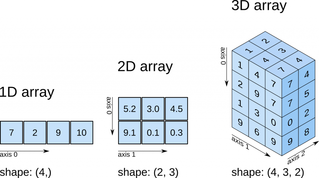
A quick note about axes in awkward: 0 is always the shallowest, while -1 is the deepest. In other words, axis=0 would tell us the number of subarrays (events), while axis=-1 would tell us the number of muons within each subarray. This array is only of dimension 2, so axis=1 or axis=-1 are the same. This usage is the same as for standard numpy arrays.
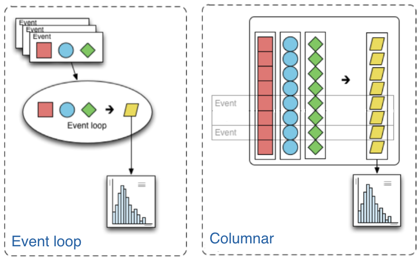
The traditional way of analyzing data in HEP involves the event loop. In this paradigm, we would write an explicit loop to go through every event (and through every field of an event that we wish to make a cut on). This method of analysis is rather bulky in comparison to the columnar approach, which (ideally) has no explicit loops at all! Instead, the fields of our data are treated as arrays and analysis is done by way of numpy-like array operations.
Most simple cuts can be handled by masking. A mask is a Boolean array which is generated by applying a condition to a data array. For example, if we want only muons with pT > 10, our mask would be:
print(muon_pt > 10)
[[True, False], [True], [True, False, False], ... [True], [True], [True, False]]
Then, we can apply the mask to our data. The syntax follows other standard array selection operations: data[mask]. This will pick out only the elements of our data which correspond to a True.
Our mask in this case must have the same shape as our muons branch, and this is guaranteed to be the case since it is generated from the data in that branch. When we apply this mask, the output should have the same amount of events, but it should down-select muons - muons which correspond to False should be dropped. Let’s compare to check:
print('Input:', muon_pt)
print('Output:', muon_pt[muon_pt > 10])
Input: [[53.4, 0.792], [30.1], [32.9, 0.769, 0.766], ... 40], [37.9], [35.2], [30.9, 3.59]]
Output: [[53.4], [30.1], [32.9], [28.3], [41.7], ... [42.6], [40], [37.9], [35.2], [30.9]]
We can also confirm we have fewer muons now, but the same amount of events:
print('Input Counts:', ak.sum(ak.num(muon_pt, axis=1)))
print('Output Counts:', ak.sum(ak.num(muon_pt[muon_pt > 10], axis=1)))

print('Input Size:', ak.num(muon_pt, axis=0))
print('Output Size:', ak.num(muon_pt[muon_pt > 10], axis=0))
Input Counts: 26690
Output Counts: 17274

Input Size: 15090
Output Size: 15090
Challenge!
How many muons have a transverse momentum (
pt) greater than 30 GeV/c?Revisit the output of
event.keys(). How many jets in total were produced and how many have a transverse momentum greater than 30 GeV/c?Solution
We modify the above code to mask the muons with
muon_pt> 30. We also make use of thejet_ptvariable to perform a similar calculation.print('Input Counts:', ak.sum(ak.num(muon_pt, axis=1))) print('Output Counts:', ak.sum(ak.num(muon_pt[muon_pt > 30], axis=1)))Input Counts: 26690 Output Counts: 13061jet_pt = events['jet_pt'].array() print('Input Counts:', ak.sum(ak.num(jet_pt, axis=1))) print('Output Counts:', ak.sum(ak.num(jet_pt[jet_pt > 30], axis=1))) print('Input Counts:', ak.num(jet_pt, axis=0)) print('Output Counts:', ak.num(jet_pt[jet_pt > 30], axis=0))Input Counts: 26472 Output Counts: 19419 Input Counts: 15090 Output Counts: 15090So we find that there are 13061 muons, taken from these 15090 proton-proton collisions that have transverse momentum greater than 30 GeV/c.
Similarly we find that there are 26472 jets, taken from these 15090 proton-proton collisions, and 19419 of them have transverse momentum greater than 30 GeV/c.
Let’s quickly make a simple histogram with the widely used matplotlib library. First we will import it.
import matplotlib.pylab as plt
When we make our histogram, we need to first “flatten” the awkward aray before passing it to matplotlib.
This is because matplotlib doesn’t know how to handle the jagged nature of awkward arrays.
# Flatten the jagged array before we histogram it
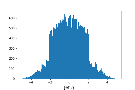
values = ak.flatten(events['jet_eta'].array())
fig = plt.figure(figsize=(6,4))
plt.hist(values,bins=100,range=(-5,5))
plt.xlabel(f'Jet $\eta$',fontsize=14)
;
(The semi-colon at the end of the code is just to suppress the output of whatever the last line of the python code in the cell.)
Output of
jet_etahistogram
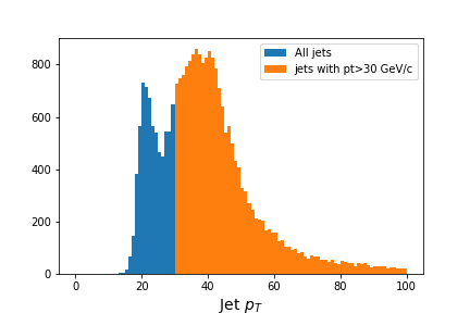
And here’s how we could use the mask in our plot.
# Flatten the jagged array before we histogram it
fig = plt.figure(figsize=(6,4))

values = ak.flatten(jet_pt)

plt.hist(values,bins=100,range=(0,100), label='All jets')
plt.hist(values[values>30],bins=100,range=(0,100), label='jets with pt>30 GeV/c')

plt.xlabel(f'Jet $p_T$',fontsize=14)
plt.legend()
;
Output of
jet_pthistogram with and without mask
Coffea
Awkward arrays let us access data in a columnar fashion, but that’s just the first part of doing an analysis. Coffea builds upon this foundation with a variety of features that better enable us to do our analyses. These features include:
-
Hists give us ROOT-like histograms. Actually, this is now a standalone package, but it has been heavily influenced by the (old) coffea hist subpackage, and it’s a core component of the coffea ecosystem.
-
NanoEvents and Schemas allows us to apply a schema to our awkward array. This schema imposes behavior that we would not have in a simple awkward array, but which makes our (HEP) lives much easier. On one hand, it can serve to better organize our data by providing a structure for naming, nesting, and cross-referencing fields; it also allows us to add physics object methods (e.g., for LorentzVectors).
-
Processors are coffea’s way of encapsulating an analysis in a way that is deployment-neutral. Once you have a Coffea analysis, you can throw it into a processor and use any of a variety of executors (e.g. Dask, Parsl, Spark) to chunk it up and run it across distributed workers. This makes scale-out simple and dynamic for users.
-
Lookup tools are available in Coffea for any corrections that need to be made to physics data. These tools read a variety of correction file formats and turn them into lookup tables.
In summary, coffea’s features enter the analysis pipeline at every step. They improve the usability of our input (NanoEvents), enable us to map it to a histogram output (Hists), and allow us tools for scaling and deployment (Processors).
Coffea NanoEvents and Schemas: Making Data Physics-Friendly
Before we can dive into our example analysis, we need to spruce up our data a bit.
Let’s turn our attention to NanoEvents and schemas. Schemas let us better organize our file and impose physics methods onto our data. There exist schemas for some standard file formats, most prominently NanoAOD (which will be, in the future, the main format in which CMS data will be made open), and there is a BaseSchema which operates much like uproot. The coffea development team welcomes community development of other schemas.
For the purposes of this tutorial, we already have a schema. Again, this was prepared already by Mat Adamec for the IRIS-HEP AGC Workshop 2022. Here, however, we will try to go into the details.
Before we start, don’t forget to include the libraries we need, including now the coffea ones:
import uproot
import awkward as ak
import hist
from hist import Hist
from coffea.nanoevents import NanoEventsFactory, BaseSchema
Remember the output we had above. After loading the file, we saw a lot of branches. Let’s zoom in on the muon-related ones here:
'numbermuon', 'nmuon_e', 'muon_e', 'nmuon_pt', 'muon_pt', 'nmuon_px', 'muon_px', 'nmuon_py', 'muon_py', 'nmuon_pz', 'muon_pz', 'nmuon_eta', 'muon_eta', 'nmuon_phi', 'muon_phi', 'nmuon_ch', 'muon_ch', 'nmuon_isLoose', 'muon_isLoose', 'nmuon_isMedium', 'muon_isMedium', 'nmuon_isTight', 'muon_isTight', 'nmuon_isSoft', 'muon_isSoft', 'nmuon_isHighPt', 'muon_isHighPt', 'nmuon_dxy', 'muon_dxy', 'nmuon_dz', 'muon_dz', 'nmuon_dxyError', 'muon_dxyError', 'nmuon_dzError', 'muon_dzError', 'nmuon_pfreliso03all', 'muon_pfreliso03all', 'nmuon_pfreliso04all', 'muon_pfreliso04all', 'nmuon_pfreliso04DBCorr', 'muon_pfreliso04DBCorr', 'nmuon_TkIso03', 'muon_TkIso03', 'nmuon_jetidx', 'muon_jetidx', 'nmuon_genpartidx', 'muon_genpartidx', 'nmuon_ip3d', 'muon_ip3d', 'nmuon_sip3d', 'muon_sip3d'
By default, uproot (and BaseSchema) treats all of the muon branches as distinct branches with distinct data. This is not ideal, as some of our data is redundant, e.g., all of the nmuon_* branches better have the same counts. Further, we’d expect all the muon_* branches to have the same shape, as each muon should have an entry in each branch.
The first benefit of instating a schema, then, is a standardization of our fields. It would be more succinct to create a general muon collection under which all of these branches (in NanoEvents, fields) with identical size can be housed, and to scrap the redundant ones. We can use numbermuon to figure out how many muons should be in each subarray (the counts, or offsets), and then fill the contents with each muon_* field. We can repeat this for the other branches.
We will, however, use a custom schema called AGCSchema, whose implementation resides in the agc_schema.py file you just downloaded.
Let’s open our example file again, but now, instead of directly using uproot, we use the AGCSchema class.
from agc_schema import AGCSchema
agc_events = NanoEventsFactory.from_root('root://eospublic.cern.ch//eos/opendata/cms/upload/od-workshop/ws2021/myoutput_odws2022-ttbaljets-prodv2.0_merged.root', schemaclass=AGCSchema, treepath='events').events()
For NanoEvents, there is a slightly different syntax to access our data. Instead of querying keys() to find our fields, we query fields. We can still access specific fields as we would navigate a dictionary (collection[field]) or we can navigate them in a new way: collection.field.
Let’s take a look at our fields now:
agc_events.fields
['muon', 'fatjet', 'jet', 'photon', 'electron', 'tau', 'met', 'trig', 'btag', 'PV']
We can confirm that no information has been lost by querying the fields of our event fields:
agc_events.muon.fields
['pt', 'px', 'py', 'pz', 'eta', 'phi', 'ch', 'isLoose', 'isMedium', 'isTight', 'isSoft', 'isHighPt', 'dxy', 'dz', 'dxyError', 'dzError', 'pfreliso03all', 'pfreliso04all', 'pfreliso04DBCorr', 'TkIso03', 'jetidx', 'genpartidx', 'ip3d', 'sip3d', 'energy']
So, aesthetically, everything is much nicer. If we had a messier dataset, the schema can also standardize our names to get rid of any quirks. For example, every physics object property in our tree has an n* variable which, if you were to check their values, you would realize that they repeat. They give just the number of objects in the field. We need only one variable to check that, and for the muons would be numbermuon. This sort of features are irrelevant after the application of the schema, so we don’t have to worry about it.
There are also other benefits to this structure: as we now have a collection object (agc_events.muon), there is a natural place to impose physics methods. By default, this collection object does nothing - it’s just a category. But we’re physicists, and we often want to deal with Lorentz vectors. Why not treat these objects as such?
This behavior can be built fairly simply into a schema by specifying that it is a PtEtaPhiELorentzVector and having the appropriate fields present in each collection (in this case, pt, eta, phi and e). This makes mathematical operations on our muons well-defined:
agc_events.muon[0, 0] + agc_events.muon[0, 1]
<LorentzVectorRecord ... y: -17.7, z: -11.9, t: 58.2} type='LorentzVector["x": f...'>
And it gives us access to all of the standard LorentzVector methods, like \(\Delta R\):
agc_events.muon[0, 0].delta_r(agc_events.muon[0, 1])
2.512794926098977
We can also access other LorentzVector formulations, if we want, as the conversions are built-in:
agc_events.muon.x, agc_events.muon.y, agc_events.muon.z, agc_events.muon.mass
/usr/local/venv/lib/python3.10/site-packages/awkward/_connect/_numpy.py:195: RuntimeWarning: invalid value encountered in sqrt
  result = getattr(ufunc, method)(
(<Array [[50.7, 0.0423], ... [21.1, -1.38]] type='15090 * var * float32'>, <Array [[-16.9, -0.791], ... [-22.6, 3.31]] type='15090 * var * float32'>, <Array [[-7.77, -4.14], ... [-11, -6.83]] type='15090 * var * float32'>, <Array [[0.103, 0.106], ... [0.105, 0.106]] type='15090 * var * float32'>)
NanoEvents can also impose other features, such as cross-references in our data; for example, linking the muon jetidx to the jet collection. This is not implemented in our present schema.
Let’s take a look at the agc_schema.py file
Anyone, in principle, can write a schema that suits particular needs and that could be plugged into the coffea insfrastructure. Here we present a challenge to give you a feeling of the kind of arrangements schemas can take care of.
Challenge: Finding the corrected jet energy in the LorentzVector
If you check the variables above, you will notice that the
jetobject has an energyerecorded but also, as you learn from the physics objects lesson,corre, which is the corrected energy. You can also realize about this if you dump the fields for the jet:agc_events.jet.fieldsYou should find that you can see the
correvariable.Inspect and study the file
agc_schema.pyto see how thecorreenergy was added as the energy to the LorentzVector and not the uncorrectedeenergy. The changes for_eshould remain valid for the rest of the objects though. Note that you could correct for thefatjetalso in the same line of action.
Overnight challenge! Make your own plot!
You’ve now seen how to make basic plots of the variables in these ROOT files, as well as how to mask the data based on other variables.
You are challenged to make at least one plot, making use of the data file and tools we learned about in this lesson. It doesn’t matter what it is…you can even just reproduce the plots we asked you to make in this lesson. To save the plot, you’ll want to add something like the following line of code after you make any of the plots.
plt.savefig('my_plot.png')The figure will show up in the directory in both docker and on your local machine.
When you get the image, you can add it to these Google Slides.
Good luck! And we’ll pick this up tomorrow!
Key Points
Understanding the basic physics will help you understand how to translate physics into computer code.
We will be perfoming a real but simplified HEP analysis using CMS Run2 open data using columnar analysis.
Coffea is a framework which builds upons several tools to make columnar analysis more efficient in HEP.
Schemas are a simple way of rearranging our data content so it is easier to manipulate