Pre-lesson reading and computational setup

Overview

Teaching: 30 min
Exercises: 20 min

Questions

• What analysis will we be doing?

Objectives

• Skim the paper on which this lesson is based.

• Make sure your computing environment is setup properly

Physics introduction

In this lesson, you will be walked through a mini-reproduction of a 2017 analysis from the CMS collaboration. The cross-section for the production of top-quark / anti-top-quark pairs in proton-proton collisions was measured. Put another way, we measured the probability that a top-quark and an anti-top quark pair are produced when protons are collided at a center-of-mass energy of 13 TeV.

.

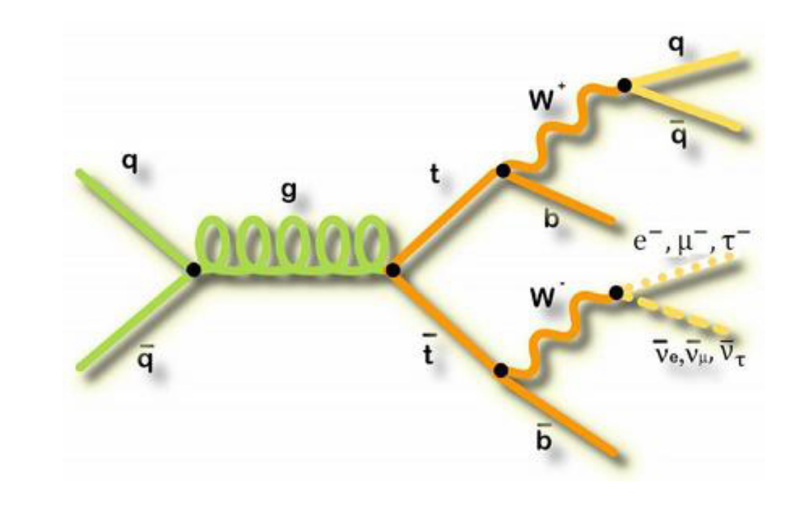
To go into a bit more detail in this simplified analysis we will be working towards a measurement of the top and anti-top quark production cross section \(\sigma_{t\bar{t}}\). The data are produced in proton-proton collisions at \(\sqrt{s}\) = 13 TeV at the beginning of Run 2 of the LHC. We will be examining the lepton+jets final state \(t\bar{t} \rightarrow (bW^{+})(\bar{b}W_{-}) \rightarrow bq\bar{q} bl^{-}\bar{\nu_{l}}\) which is characterized by one lepton (here we look at electrons and muons only), significant missing transverse energy, and four jets, two of which are identified as b-jets.

Depending on how much background you have, try to read or at least skim the paper and see how much you can get out of it. We’ll discuss it in more detail in our first episode when we meet.

Set up your computing environment.

We will attempt to use tools that are built on modern, powerful and efficient python ecosystems. In particular, we will use the Columnar Object Framework For Effective Analysis (Coffea), which will provide us with basic tools and wrappers for enabling not-too-alien syntax when running columnar Collider HEP analysis.

Start up Docker and JupyterLab

Type out the following commands for this episode!

For this next section, you’ll be asked to type out the provided commands in a Jupyter notebook, a popular development environment that allows you to use python in an interactive way.

Please enter in these commands yourself for this episode.

To create or run these notebooks, we will

• Start the python docker container
• Install some necessary extra module (this only needs to be done once)
• Launch Jupyter Lab, an application that makes it easier to work with Jupyter Notebooks
• Create a new Jupyter Notebook for this episode.

Start Docker If you have already successfully installed and run the Docker example with python tools, then you need only execute the following command.

docker start -i my_python  #give the name of your container

If this doesn’t work, return to the python tools Docker container lesson to work through how to start the container.

Install the extra libraries

(If you did this already by following the setup section of this lesson, then you needn’t do this part again.)

In order to use the coffea framework for our analysis, we need to install these additional packages directly in our container. We are adding cabinetry as well because we will use it later in our last episode. This can take a few minutes to install.

pip install vector hist mplhep coffea cabinetry

Also, download this file, which is our starting schema. Directly in your /code area (or locally in your cms_open_data_python directory) you can simply do:

wget  https://raw.githubusercontent.com/cms-opendata-workshop/workshop2022-lesson-ttbarljetsanalysis-payload/master/trunk/agc_schema.py

Launch Jupyter Lab In your docker python container, type the following.

jupyter-lab --ip=0.0.0.0 --no-browser

Launching Jupyter Lab

You should see something like this in your Docker container terminal when you type the above jupyter-lab command.

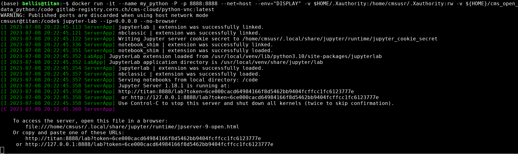
In the image above you can see the output when I start jupyter-lab on my computer. Yours won’t say exactly the same thing, but it should be similar. Take note of the last two lines that start with http://. Start up a browser locally on your laptop or desktop (not from the Docker container). Copy one of those URLs and paste it into the browser. If the first URL doesn’t work, try the other.

If it works you’ll see something in your browser similar to the following image!

Launching Jupyter Lab

If Jupyter Lab launched, you’ll see something like this.

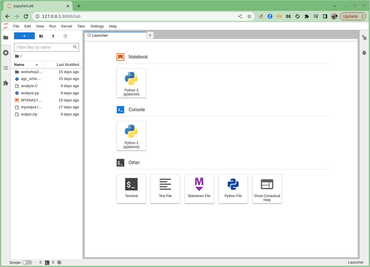
Great! You’re all set to begin the analysis!

Key Points

• Get ready for the lesson as a whole