Prep-work: Warming up for the Higgs to Ditau analysis
Overview
Teaching: 0 min
Exercises: 0 minQuestions
What will we do during this lesson?
What should I do before the lesson starts tomorrow?
Objectives
Learn a little about the analysis example we will try to reproduce during the Analysis flow lessons tomorrow
Prepare the newer-version ROOT container (or environment), which will speed things up
Overview and some requested reading
Tomorrow, we will try to use most of what you have been learning and reproduce an analysis which has been already replicated using open data in a simplified way. You will find that you have been already thinking about it in previous lessons. Please, read the very short description of this analysis. You will notice, at the bottom of that page, that there is already some code written to perform this study. However, it uses mostly a ROOT class called RDataFrame, which is a great tool to perform columnar analysis, but it is maybe not very well suited for a first approach. We invite you to got through this code quickly and try to identify the different selection cuts that are applied. We will be re-implementing these selection criteria using an event loop analysis (which is more intuitive) rather than the columnar approach.
The lesson’s activities
As with the other lessons, tomorrow’s lesson on analysis flow will have essentially three parts. In the first one we will go together through a demonstration. It is not mandatory to follow or copy every single step, but you are invited to do so if you wish. For the second part, the hands-on one, you will work on your own with instructions provided in this lesson. Instructors and facilitators will be there to answer questions. Lastly, you will be presented with an offline challenge. They day after tomorrow we will present a proposed solution to the challenge and have some time for questions and discussions.
Copying the needed files locally
For our hands-on activity tomorrow, if you have some space, you can download the needed files from here. We very much recommend this as we need them for the final part of our analysis. Copy them over to your container or VM. Working with these files locally will really speed up the analysis and so you will not need to work with an updated ROOT version (see below). However, if you decide, for some reason, to connect remotely through xrootd, a newer version of ROOT may be needed.
Alternatively, you can copy them using the xrdcp command like:
xrdcp root://eospublic.cern.ch//eos/opendata/cms/upload/od-workshop/ws2021/Run2012B_TauPlusX.root .
xrdcp root://eospublic.cern.ch//eos/opendata/cms/upload/od-workshop/ws2021/Run2012C_TauPlusX.root .
xrdcp root://eospublic.cern.ch//eos/opendata/cms/upload/od-workshop/ws2021/DYJetsToLL.root .
xrdcp root://eospublic.cern.ch//eos/opendata/cms/upload/od-workshop/ws2021/TTbar.root .
xrdcp root://eospublic.cern.ch//eos/opendata/cms/upload/od-workshop/ws2021/W1JetsToLNu.root .
xrdcp root://eospublic.cern.ch//eos/opendata/cms/upload/od-workshop/ws2021/W2JetsToLNu.root .
xrdcp root://eospublic.cern.ch//eos/opendata/cms/upload/od-workshop/ws2021/W3JetsToLNu.root .
xrdcp root://eospublic.cern.ch//eos/opendata/cms/upload/od-workshop/ws2021/GluGluToHToTauTau.root .
xrdcp root://eospublic.cern.ch//eos/opendata/cms/upload/od-workshop/ws2021/VBF_HToTauTau.root .
About the version of ROOT for our analysis
Our lesson exercises will work just fine in our Docker or VM default environments. However, note that the version of ROOT that comes with CMSSW in those environments is a rather old version, 5.32. Therefore, upgrading our ROOT environment to a newer version will really speed things up if connecting remotely. This is due, as far as we know, to the fact that xrootd, the protocol that we use to get access to ROOT files at CERN, has been drastically improved in later versions of the program.
Alternatively (and optionally), if you have some disk space of a couple of GBs, you could copy the root files we will be needing locally. This is shown in the last section of this episode. This action will also speed things up considerably even if you choose not to upgrade your root environment (we recommend this latter approach, i.e., work with your current ROOT environment but with the locally-downloaded root files).
Getting a newer version of ROOT
If you decide to work with an upgraded version of ROOT. You can follow these instructions.
If you are working with Docker, what we will do is to create a new container based on a recent ROOT container image. You can follow the same instructions you used for creating your open data container, but instead of using the cmsopendata/cmssw_5_3_32:latest (or cmsopendata/cmssw_5_3_32_vnc:latest) image you will use a new stand-alone ROOT image. The ROOT container image can be found in the Docker hub. So, for example, for Linux, creating such a container would require a line like:
docker run -it --name myroot --net=host --env="DISPLAY" -v $HOME/.Xauthority:/home/cmsusr/.Xauthority:rw rootproject/root:latest /bin/bash
Follow the corresponding instructions for your own operating system.
In the virtual machine, you could also install a newer stack of ROOT. You can get ROOT via CVMFS through the LCG releases. All information about the releases and contained packages can be found at http://lcginfo.cern.ch. The following setup line works in the SLC6 shell and the “Outer shell” (SLC7) of the open data VM (we recommend using the Outer Shell).
source /cvmfs/sft.cern.ch/lcg/views/LCG_97/x86_64-slc6-gcc8-opt/setup.sh
You can check the root version with:
root --version
Key Points
The Higgs to tautau analysis is good example of analysis that can be done with CMS open data in a relatively easy and simplified way.
A container (or environment) with a newer version of ROOT could really speed things up.
See you tomorrow!
We will continue tomorrow
Overview
Teaching: 0 min
Exercises: 0 minQuestions
Objectives
Congratulations! You are done with the prep-work for the analysis flow lesson. Our next session will start tomorrow at 15H10 (CET)!
Key Points
Demo: Datasets, trigger and luminosity
Overview
Teaching: 25 min
Exercises: 0 minQuestions
What is the strategy for the analysis flow example?
What datasets and trigger do we need?
How do we get integrated luminosities?
How do we normalize MC simulations?
Objectives
Learn about the strategy we will follow for our analysis example.
Identify the datasets and the trigger needed.
Learn about the
brilcalctool used to extract luminosities.Remember how to normalize events from simulated datasets.
Disclaimer
The first two episodes of this lesson are a demonstration. You are welcome to follow along, but if at some point you get behind typing, do not worry, you will not be needing this section in order to continue with the hands-on activity after the break. Of course, later you can refer back to these episodes and/or its video recording.
Overview
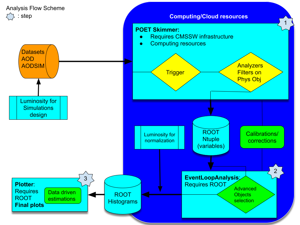
As you read yesterday, we will try to re-implement the Higgs to ditau analysis that has been already implemented but in a different fashion. The original open data analysis is based on two Github repositories. The first one is the AOD2NanoAODOutreachTool repository. There, the important piece of code is the AOD2NanoAOD.cc code. This is an analyzer, very similar to the analyzers you saw already in the POET tool. The main difference is that our POET is capable of extracting the required information in a very modular way. The second part of this analysis relies on the HiggsTauTauNanoAODOutreachAnalysis repository. The code in this repository is already independent of CMSSW but relies on ROOT libraries, some of which is rather complex for a first approach, like the usage RDataFrame class (although powerful). In summary, one has to compile and run the skim.cxx C++ code, then the histograms.py python code, and, as a last step, execute the plot.py python script. I.e., this analysis is done in 4 steps.
We will simplify this analysis by performing it in just 3 steps:
- one to skim our data out of CMSSW infrastructure
- the second one to analyze the data and produce
ROOThistograms - and the final one to make nice plots.
Later you can refer back to the original open data analysis and compare it to our more orthodox approach. We hope that adopting this more traditional method, the physics and the logic of it will be clearer.
Datasets and trigger selection
We will concentrate on studying the decays of a Higgs boson into two tau leptons in the final state of a muon lepton and a hadronically decayed tau lepton. Since we need to have tau leptons, we choose these two datasets from 2012 (we are going to use only 2012 datasets for simplicity):
- the Run2012B_TauPlusX dataset and
- the Run2012C_TauPlusX dataset.
Note the sizes of these datasets. It TBs of data. No way we can easily download or work locally with them, we would need to skim them.
For our background processes we will chose the following MC simulations:
- the DYJetsToLL dataset, which can contribute with real taus and/or misidentified leptons,
- the TTbar dataset,
- and the set of W1JetsToLNu, W2JetsToLNu, and W3JetsToLNu to complete the W+jets contribution.
As it is commonly done, we would also need to have an idea of how our signal (the process we are trying to find/discover) look like. Thus, for the Higgs production we will consider the following MC simulations:
- the GluGluToHToTauTau dataset and
- the VBF_HToTauTau dataset.
Note also that all these datasets are in the TB range.
Now, for the trigger, we will use the HLT_IsoMu17_eta2p1_LooseIsoPFTau20 as it is done in the original open data analysis. Likewise threr, we will assume that this trigger is unprescaled. Now you know, however, that one should really check that.
Luminosity calculation
One of the key aspects in any particle physics analysis is the estimation of the integrated luminosity of a given collisions dataset. From the original analysis we can see that the full integrated luminosities are:
for a total of approximately 11.5 inverse femtobarns between the two collisions datasets. But, how can we figure this out?
Fortunately we have a wonderful tool for this, called brilcalc. Here we show a simple example, but more details can be found in this CODP guide.
Installing brilcalc in your container
You can install the brilcalc tool in the same cmsopendata container that you have been using so far or even your own host machine. We will show the example using the container.
- Start your container or create a new one if you wish. We will create a fresh new one (with our own settings; feel free to change them) that we will use for the rest of this lesson (although you can recycle the one you have been using):
docker run --name analysisflow -it --net=host --env="DISPLAY" --volume="$HOME/.Xauthority:/root/.Xauthority:rw" --volume="/home/ecarrera/.ssh:/home/cmsusr/.ssh" -v "/home/ecarrera/playground:/playground" cmsopendata/cmssw_5_3_32:latest /bin/bash
- In order not to pollute the
CMSSW/srcare, we will change to the home directory:
cd ~
- Fetch the installer for the brilcalc conda environment:
wget https://cern.ch/cmslumisw/installers/linux-64/Brilconda-3.0.0-Linux-x86_64.sh
- Run the installer:
bash Brilconda-1.1.7-Linux-x86_64.sh -b -p <localbrilcondabase>
where we substitute <localbrilcondabase> with brilconda. This is the directory in which the brilcalc tools will be installed.
- Once installed successfully add the tools to your
PATHwith the following command:
export PATH=$HOME/.local/bin:$HOME/brilconda/bin:$PATH
- Then install brilcalc with this command:
pip install brilws
- Finally check by running the following:
brilcalc --version
which should output 3.6.6.
Lumi calculation example
- Now, as an example, let’s calculate the luminosity for the Run2012B_TauPlusX dataset. Let’s download the list of validated runs from this site:
wget "http://opendata.cern.ch/record/1002/files/Cert_190456-208686_8TeV_22Jan2013ReReco_Collisions12_JSON.txt"
All collision datasets have been released with a similar file. Let’s explore it:
less Cert_190456-208686_8TeV_22Jan2013ReReco_Collisions12_JSON.txt
{"190645": [[10, 110]], "190646": [[1, 111]], "190659": [[33, 167]], "190679": [[1, 55]], "190688": [[69, 249]], "190702": [[51, 53], [55, 122], [124, 169]], "190703": [[1, 252]], "190704": [[1, 3]], "190705": [[1, 5], [7, 65], [81, 336], [338, 350], [353, 383]], "190706": [[1, 126]], "190707": [[1, 237], [239, 257]], "190708": [[1, 189]], "190733": [[71, 96], [99, 389], [392, 460]], "190736": [[1, 80], [83, 185]], "190738": [[1, 130], [133, 226], [229, 349]], "190782": [[55, 181], [184, 233], [236, 399], [401, 409]], "190895": [[64, 202], [210, 302], [305, 584], [587, 948]], "190906": [[73, 256], [259, 354], [356, 496]], "190945": [[124, 207]], "190949": [[1, 81]], "191043": [[45, 46]], "191046": [[1, 21], [24, 82], [84, 88], [92, 116], [119, 180], [183, 183], [185, 239]], "191056": [[1, 1], [4, 9], [16, 17], [19, 19]], "191057": [[1, 1], [4, 40]], "191062": [[1, 1], [3, 3], [5, 214], ...
It contains the list of runs and luminosity sections in those runs that have been blessed for quality.
Note that the run range for the Run2012B_TauPlusX dataset is from run 193833 to 196531.
- Obtain the integrated luminosity:
brilcalc lumi -c web --type pxl -u /pb --begin 193833 --end 196531 -i Cert_190456-208686_8TeV_22Jan2013ReReco_Collisions12_JSON.txt > lumi.log &
#Summary:
+-------+------+-------+-------+-------------------+------------------+
| nfill | nrun | nls   | ncms  | totdelivered(/pb) | totrecorded(/pb) |
+-------+------+-------+-------+-------------------+------------------+
| 56    | 146  | 50895 | 50895 | 4493.290785044    | 4411.703590626   |
+-------+------+-------+-------+-------------------+------------------+
#Check JSON:
#(run,ls) in json but not in results: [(190645, 10), (190645, 11), (190645, 12), (190645, 13), (190645, 14), (190645, 15), (190645, 16), (190645, 17), (190645, 18), (19
0645, 19), (190645, 20), (190645, 21), (190645, 22), (190645, 23), (190645, 24), (190645, 25), (190645, 26), (190645, 27), (190645, 28), (190645, 29), (190645, 30), (19
0645, 31), (190645, 32), (190645, 33), (190645, 34), (190645, 35), (190645, 36), (190645, 37), (190645, 38), (190645, 39), (190645, 40), (190645, 41), (190645, 42), (19
0645, 43), (190645, 44), (190645, 45), (190645, 46), (190645, 47), (190645, 48), (190645, 49), (190645, 50), (190645, 51), (190645, 52), (190645, 53), (190645, 54), (19
0645, 55), (190645, 56), (190645, 57), (190645, 58), (190645, 59), (190645, 60), (190645, 61), (190645, 62), (190645, 63), (190645, 64), (190645, 65), (190645, 66), (19
0645, 67), (190645, 68), (190645, 69), (190645, 70), (190645, 71), (190645, 72), (190645, 73), (190645, 74), (190645, 75), (190645, 76), (190645, 77), (190645, 78), (19
0645, 79), (190645, 80), (190645, 81), (190645, 82), (190645, 83), (190645, 84), (190645, 85), (190645, 86), (190645, 87), (190645, 88), (190645, 89), (190645, 90), (19
0645, 91), (190645, 92), (190645, 93), (190645, 94), (190645, 95), (190645, 96), (190645, 97), (190645, 98), (190645, 99), ....
which is exactly the number quoted in the original analysis.as we will see later.
Note: You may notice, at the end of the output, luminosity sections that are listed in the json quality file but do not have any luminosity values corresponding to them. These correspond to sections that are left-overs at the end of a run, which where still tagged as STABLE RUN, but actually did not provide any luminosity. These are safe to ignore as they do not contain any events.
Normalization of MC simulations
Whether it is your signal or background process, when it comes to MC simulations there is a key aspect to take into account. Given the process cross section, and the integrated luminosity from collisions data, how many events will you have to simulate and/or use in order to make a good comparison with your data? A key ingredient to answer this question is the scale factor you will have to apply in order to normalize the contribution.
As you may know, the number of events (N) of a given process (with cross section sigma) that are approximately expected to be found in a collisions dataset with integrated luminosity (L) is:
If you happen to simulate Nmc events of a given process with cross section sigma, then to properly normalize this contribution to the known integrated luminosity you need :
I.e., the factor we are looking for is
One should consider this when designing a simulation production (not covered in this workshop but possible with CMS open data infrastructure), and to normalize the simlated datasets already available (we will do this later in the lesson.)
Key Points
A simplified analysis can be done with all the open data tools we have learned so far.
We will be using collisions data from 2012 and several MC simulated datasets.
brilcalcis a tool for estimating integrated luminosities (and can be also used for obtaining other information like trigger prescales.)
Demo: Skimming
Overview
Teaching: 20 min
Exercises: 0 minQuestions
Do we skim our data before perfoming the analysis study?
How can I skim datasets efficiently with CMSSW
Objectives
Justify the need for large scale skimming
Lear how to best skim a dataset using CMSSW EDFilters
Disclaimer
The first two episodes of this lesson are a demonstration. You are welcome to follow along, but if at some point you get behind typing, do not worry, you will not be needing this section in order to continue with the hands-on activity after the break. Of course, later you can refer back to these episodes and/or its video recording.
Introduction
So, we are now ready to start out analysis example. We will go from very early datasets (in AOD format) to nice plots.
As you saw, the sizes of the datasets we are interested in are massive. Obviously, we do not need all the information that is stored in all of those AOD files. We should find a way then to cherry-pick only the fruit we need, i.e., those objects that we are interested in. For our Higgs to ditau analysis, it will be essentially muons, taus and some missing energy (we do have neutrinos in our decays).
Physics for POETs
You have been exploring ways (implemented in code) of accessing the information we need from physics objects. In particular, you have worked already with the POET repository. For this demonstration we will use our fresh container (used in the last episode) and check out this repository. You can recycle the POET you already have in your container if you want to explore along with us:
git clone git://github.com/cms-legacydata-analyses/PhysObjectExtractorTool.git
As the instructions recommend, we need to get into the PhysObjectExtractor package, and compile:
cd PhysObjectExtractorTool/PhysObjectExtractor
scram b
Let’s take a quick look at the configuration file, and in the process we will be identifying some of the modules that will be important for us:
less python/poet_cfg.py
A few things we can see:
- The number of events is just
200 - The source file feeding the PoolSource module is that: just one file. We would really need to run over the whole dataset (and not only one dataset but several.)
- There is some utility, called
FileUtilsthat could be useful to load not only one but several root files through index lists, like the ones found in each dataset’s pages, e.g. - For collisions data, there is also a module which checks whether the data was quality-blessed through the
jsonfile runs and lumi sections listing. - Aside from all the modules that configure the different analyzers, there are a couple of modules labeled as
Filters, which are commented out. We will use them in a moment, but first, let’s make just one simple change and run.
We will activate the FileUtils module, replacing the one-file approach that comes as default. So, after the change to config file, the corresponding section will look like:
#---- Define the test source files to be read using the xrootd protocol (root://), or local files (file:)
#---- Several files can be comma-separated
#---- A local file, for testing, can be downloaded using, e.g., the cern open data client (https://cernopendata-client.readthedocs.io/en/latest/):
#---- python cernopendata-client download-files --recid 6004 --filter-range 1-1
#---- For running over larger number of files, comment out this section and use/uncomment the FileUtils infrastructure below
#if isData:
#       sourceFile='root://eospublic.cern.ch//eos/opendata/cms/Run2012B/DoubleMuParked/AOD/22Jan2013-v1/10000/1EC938EF-ABEC-E211-94E0-90E6BA442F24.root'
#else:
#       sourceFile='root://eospublic.cern.ch//eos/opendata/cms/MonteCarlo2012/Summer12_DR53X/TTbar_8TeV-Madspin_aMCatNLO-herwig/AODSIM/PU_S10_START53_V19-v2/00000/000A$
#process.source = cms.Source("PoolSource",
#    fileNames = cms.untracked.vstring(
#        #'file:/playground/1EC938EF-ABEC-E211-94E0-90E6BA442F24.root'
#       sourceFile
#    )
#)

#---- Alternatively, to run on larger scale, one could use index files as obtained from the Cern Open Data Portal
#---- and pass them into the PoolSource.  The example is for 2012 data
files = FileUtils.loadListFromFile("data/CMS_Run2012B_DoubleMuParked_AOD_22Jan2013-v1_10000_file_index.txt")
files.extend(FileUtils.loadListFromFile("data/CMS_Run2012B_DoubleMuParked_AOD_22Jan2013-v1_20000_file_index.txt"))
files.extend(FileUtils.loadListFromFile("data/CMS_Run2012B_DoubleMuParked_AOD_22Jan2013-v1_20001_file_index.txt"))
files.extend(FileUtils.loadListFromFile("data/CMS_Run2012B_DoubleMuParked_AOD_22Jan2013-v1_20002_file_index.txt"))
files.extend(FileUtils.loadListFromFile("data/CMS_Run2012B_DoubleMuParked_AOD_22Jan2013-v1_210000_file_index.txt"))
files.extend(FileUtils.loadListFromFile("data/CMS_Run2012B_DoubleMuParked_AOD_22Jan2013-v1_30000_file_index.txt"))
files.extend(FileUtils.loadListFromFile("data/CMS_Run2012B_DoubleMuParked_AOD_22Jan2013-v1_310000_file_index.txt"))
process.source = cms.Source(
    "PoolSource", fileNames=cms.untracked.vstring(*files))
We will also activate the reading of local DB files so the process goes faster:
#---- These two lines are needed if you require access to the conditions database. E.g., to get jet energy corrections, trigger prescales, etc.
process.load('Configuration.StandardSequences.FrontierConditions_GlobalTag_cff')
process.load('Configuration.StandardSequences.Services_cff')
#---- Uncomment and arrange a line like this if you are getting access to the conditions database through CVMFS snapshot files (requires installing CVMFS client)
#process.GlobalTag.connect = cms.string('sqlite_file:/cvmfs/cms-opendata-conddb.cern.ch/FT53_V21A_AN6_FULL.db')
#---- The global tag must correspond to the needed epoch (comment out if no conditions needed)
#if isData: process.GlobalTag.globaltag = 'FT53_V21A_AN6::All'
#else: process.GlobalTag.globaltag = "START53_V27::All"
#---- If the container has local DB files available, uncomment lines like the ones below
#---- instead of the corresponding lines above
if isData: process.GlobalTag.connect = cms.string('sqlite_file:/opt/cms-opendata-conddb/FT53_V21A_AN6_FULL_data_stripped.db')
else:  process.GlobalTag.connect = cms.string('sqlite_file:/opt/cms-opendata-conddb/START53_V27_MC_stripped.db')
if isData: process.GlobalTag.globaltag = 'FT53_V21A_AN6_FULL::All'
else: process.GlobalTag.globaltag = "START53_V27::All"
The index files are in the
datadirectory. Also, in that directory, you will find other index files and data quality json files. Also, note that the cfg file is not perfect: theisDataflag does not control the execution over collisions or simulation index files any more, so you have to be careful about it.
Now, let’s run:
cmsRun python/poet_cfg.py True True > full.log 2>&1 &
While this completes, let us remember what this code is doing; essentially, executing all routines necessary to get information about the different physics objects, e.g.:
#---- Finally run everything!
#---- Separation by * implies that processing order is important.
#---- separation by + implies that any order will work
#---- One can put in or take out the needed processes
if doPat:
        process.p = cms.Path(process.patDefaultSequence+process.myevents+process.myelectrons+process.mymuons+process.myphotons+process.myjets+process.mymets+process.my...
else:
     	if isData: process.p = cms.Path(process.myevents+process.myelectrons+process.mymuons+process.myphotons+process.myjets+process.mymets+process.mytaus+process.myt...
        else: process.p = cms.Path(process.selectedHadronsAndPartons * process.jetFlavourInfosAK5PFJets * process.myevents+process.myelectrons+process.mymuons+process..
The output we get weights 5.2MB:
ls -ltrh
-rw-r--r-- 1 cmsusr cmsusr 5.2M Jul 19 04:29 myoutput.root
To Filter or not to filter
Let’s do a very crude estimate. If you remember, this file had 12279 events. Since we processed
200, running over the whole file would result in amyoutput.rootfile of5.2*12279/200~320MB. Accoring to this dataset’s record, there are2279files. It means that the final processing of this dataset will be~730GB. Since we have to process several datasets, this is just very difficult.
So we need some sort of filtering. For this workshop, we need to either access the output files remotely, via xrootd, or download them locally. Being able to do so, depends on the final sizes. We could probably store larger files somewhere in the cloud, but the access will also be more difficult, slower and costly. For this reason, we will filter hard on our dataset.
We call this act of filtering the data, skimming. CMSSW hast specific tools, called EDFilters to do this job. They could look very much like an EDAnalyzer, but they filter events rather than analyze them.
Take a look at the src area of the PhysObjectExtractor package:
ls -1 src
ElectronAnalyzer.cc
EventAnalyzer.cc
GenParticleAnalyzer.cc
JetAnalyzer.cc
MetAnalyzer.cc
MuonAnalyzer.cc
PatJetAnalyzer.cc
PhotonAnalyzer.cc
SimpleMuTauFilter.cc
TauAnalyzer.cc
TrackAnalyzer.cc
TriggObjectAnalyzer.cc
TriggerAnalyzer.cc
VertexAnalyzer.cc
Notice the one filter example in the crowd: the SimpleMuTauFilter.cc. Of course, it was one designed with the workshop in mind. Let’s take a look at it. You will see that it filters in the pT and eta variable for muons and taus and some other qualities. In the original analysis of Higgs to ditau, this corresponds to the first few selection cuts (except for the trigger requirement).
There is another filter, which we could in principle use to filter on the trigger. However, we will keep the trigger information for later processing, just to show its usage. Now, let us activate the SimpleMuTauFilterin the configuration file. We will have to uncomment these line:
#---- Example of a CMSSW filter that can be used to cut on a given set of triggers
#---- This filter, however, does know about prescales
#---- A previous trigger study would be needed to cut hard on a given trigger or set of triggers
#---- The filter can be added to the path below if needed but is not applied by default
#process.load("HLTrigger.HLTfilters.hltHighLevel_cfi")
#process.hltHighLevel.HLTPaths = cms.vstring('HLT_IsoMu17_eta2p1_LooseIsoPFTau20_v*')


#---- Example of a very basic home-made filter to select only events of interest
#---- The filter can be added to the running path below if needed but is not applied by default
process.mutaufilter = cms.EDFilter('SimpleMuTauFilter',
                                  InputCollectionMuons = cms.InputTag("muons"),
                                   InputCollectionTaus = cms.InputTag("hpsPFTauProducer"),
                                   mu_minpt = cms.double(17),
                                   mu_etacut = cms.double(2.1),
                                   tau_minpt = cms.double(20),
                                   tau_etacut = cms.double(2.3)
                                   )
Finally, let’s put it to work in the final CMSSW path that will be executed:
#---- Finally run everything!
#---- Separation by * implies that processing order is important.
#---- separation by + implies that any order will work
#---- One can put in or take out the needed processes
if doPat:
	process.p = cms.Path(process.mutaufilter+process.patDefaultSequence+process.myevents+process.myelectrons+process.mymuons+process.myphotons+process.myjets+process.mymets+process.mytaus+process.mytrigEvent+process.mypvertex+process.mytracks+process.mygenparticle+process.mytriggers)
else:
	if isData: process.p = cms.Path(process.myevents+process.myelectrons+process.mymuons+process.myphotons+process.myjets+process.mymets+process.mytaus+process.mytrigEvent+process.mypvertex+process.mytracks+process.mygenparticle+process.mytriggers)
	else: process.p = cms.Path(process.selectedHadronsAndPartons * process.jetFlavourInfosAK5PFJets * process.myevents+process.myelectrons+process.mymuons+process.myphotons+process.myjets+process.mymets+process.mytaus+process.mytrigEvent+process.mypvertex+process.mytracks+process.mygenparticle+process.mytriggers)
Let’s run again to see what happens to the file size:
python python/poet_cfg.py #always good to check for syntax
cmsRun python/poet_cfg.py True True > filter.log 2>&1 &
The output we get weights just 22K:
-rw-r--r-- 1 cmsusr cmsusr 22K Jul 19 06:01 myoutput.root
This is just ~0.4% of the original size (ok, maybe in this particular case, the root file could actually be empty, but the reduction is indeed of that order), which means that the full dataset could be skimmed down to ~3GB, a much more manageable size.
Based on these simple checks, you could also estimate the time it would take to run over all the datasets we need using a single computer. To be efficient, you will need a computer cluster, but we will leave that for the Cloud Computing lesson. Fortunately, we have prepared these skims already at CERN, using CERN/CMS computing infrastructure. The files you will find at this place (you probably already downloaded them during the prep-work) were obtained in essentially the same way, except that we dropped out objects like jets, photons, and trigEvent, which we won’t be needing for this simple exercise.
Note that, at this point, you could decide to use an alternative way storing the output. You could, for instance, decide to just dump a simple csv file with the information you need, or use another commercial library to change to a different output format. We will continue, however, using the
ROOTformat, just because this is what we are familiar with and it will allow us to get some nice plots.
This completes the first step of the analysis chain.
Key Points
One of the earlier steps in a particle physics analysis with CMS open data from Run 1 would be to skim the datasets down to a manageable size
CMSSW offers a simple an efficient way of doing so.
Skimming usually requires decent computing resources and/or time.
Break
Overview
Teaching: 0 min
Exercises: 15 minQuestions
Objectives
Break well-deserved, we will see you again in 15’ for the hands-on part of the lesson.
Key Points
Hands-on: EventLoopAnalysisTemplate
Overview
Teaching: 0 min
Exercises: 40 minQuestions
What kind of anlaysis code should I use for analyzing flat ROOT nuples?
How can I build such a code?
Objectives
Learn the most simple way of accessing information from a ROOT flat ntuple file
Lear how to build a analysis skeleton
Disclaimer
During the hands-on sessions, there will be less talking from our side and more reading from yours. You should try to follow the instructions below in detail. If something is not clear, we are here to help. We will try to silently work on the same exercises as you, so we can keep up with possible questions or discussion.
What to do with the skimmed files
Ok, we got these files from here, now what?
- DYJetsToLL.root
- GluGluToHToTauTau.root
- Run2012B_TauPlusX.root
- Run2012C_TauPlusX.root
- TTbar.root
- VBF_HToTauTau.root
- W1JetsToLNu.root
- W2JetsToLNu.root
- W3JetsToLNu.root
Well, we need to do some analysis. I.e., we would like to apply selection cuts, make some checks maybe (if we were more serious, apply some corrections, calibrations, etc) before selecting some variables of interest and producing histograms. Just for references, comparing this to the original RDataFrame analysis, we would like to apply most of the selection criteria here and here so we can later use a modified version of this python script to make pretty plots. Of course these is a toy analysis. If you read the original publication, it has more selection requirements and include more decay channels.
In order to access the information stored now in the myoutput.root-kind of files (remember that they are the output of the POET), we need again some C++ code. The advantage of these files (over the AOD files before) is that they are essentially flat (we call them ntuples), i.e., they do not generally have a crazy/complicated structure like the AOD files (for which you required CMSSW libraries). They just need ROOT libraries to be analyzed. For this reason, and maybe this is a drawback, you do need ROOT.
Fortunately, you can work in your good old cmssw-opendata container (which has an old version of ROOT) or you could use a stand-alone ROOT container, like it was explained in the prep-work lesson.
We will stick to the cmssw-opendata container because we downloaded already the files above. If you couldn’t download them, it is possible to have access remotely, using the xrootd protocol, but this will be rather slow unless you are working on a newer ROOT stand-alone container. In any case the files are available at root://eospublic.cern.ch//eos/opendata/cms/upload/od-workshop/ws2021/
Getting a code skeleton for analysis
ROOT class, TTree, has some nice nice methods that can be used to extract a code skeleton. Let’s explore this just a bit and then we will present you with a fully functional template for our analysis.
Let’s try to open one of our skimmed files above. First jump-start your container and/or VM like you usually do (if you continue from the Demo episodo, then you do not have to do anything else):
docker start -i <name of container>
It would be best to move to the PhysObjectExtractorTool/PhysObjectExtractor/test/ (although this is not required):
cd PhysObjectExtractorTool/PhysObjectExtractor/test/
ROOT-open one of these files:
root -l Run2012B_TauPlusX.root
(or root -l root://eospublic.cern.ch//eos/opendata/cms/upload/od-workshop/ws2021/Run2012B_TauPlusX.root, if you are trying to access them remotely)
Let’s create a pointer to one of the Events tree in one of the directories (let’s choose muons), and then execute the MakeClass() method to obtain a code skeleton and then exit ROOT. We are naming the resulting C++ code simply “muons”
Attaching file Run2012B_TauPlusX.root as _file0...
root [1] TTree* tmuons = (TTree*)_file0->Get("mymuons/Events");
root [2] tmuons->MakeClass("muons")
Info in <TTreePlayer::MakeClass>: Files: muons.h and muons.C generated from TTree: Events
(Int_t)0
root [3] .q
This will generate a C++ Class with a header file, muons.h, and a source file, muons.C. Open these files and explore them quickly, try to make sense of what you see, but do not spend too much time on them. You will find that they are basically an empty skeleton with declarations and definitions that can be used to read the variables stored in our ntuple files, like Run2012B_TauPlusX.root.
Putting it all together a single analysis file
We can put the structure of these two files together and create a single analysis file, which we have call EventLoopAnalysisTemplate.cxx. This example is part of the POET infrastructure and it resides precisely in the directory you are currently at, i.e. PhysObjectExtractorTool/PhysObjectExtractor/test. You will probably have to update your repository with git pull to get the latest version. Alternatively, you can download it directly with wget https://raw.githubusercontent.com/cms-opendata-workshop/workshop2021-payload-analysisflow/master/EventLoopAnalysisTemplate.cxx
Let’s take a look and try to understand briefly how it works. Take your time and the instructor if there is something not clear. Then, we will compile and run it.
Open this EventLoopAnalysisTemplate.cxx file with an editor or simply look inside with the less command.
Since this will run compiled, let’s start with the main function:
//-----------------------------------------------------------------
int main()
{
//-----------------------------------------------------------------

  //To be able to read the trigger map
  gROOT->ProcessLine("#include<map>");


  //Compute event weights to be used for the respective datasets
  //const float integratedLuminosity = 4.412 * 1000.0; // Run2012B only
  //const float integratedLuminosity = 7.055 * 1000.0; // Run2012C only
  //const float integratedLuminosity = 11.467 * 1000.0; // Run2012B+C
  //const float mc_w = <xsec> / <#events> * integratedLuminosity;
  const float data_w = 1.0;

  map<string, pair<string,float> > sampleNames;
  //sampleNames.insert(make_pair("MCSample",make_pair("mc",mc_w)));
  sampleNames.insert(make_pair("myoutput",make_pair("data",data_w)));

  //loop over sample files with names  defined above
  for(map< string,pair<string,float> >::iterator it=sampleNames.begin();
      it!=sampleNames.end();it++){

    TString samplename = it->first;
    TString thelabel = it->second.first;
    Float_t sampleweight = it->second.second;

    TStopwatch time;
    time.Start();
    cout << ">>> Processing sample " << samplename <<" with label "<<thelabel<<" and weight "<<sampleweight<<":" <<endl;

    TString filename = samplesBasePath+samplename+".root";

    cout<<"Build the analysis object with file "<<filename<<endl;
    EventLoopAnalysisTemplate mytemplate(filename,thelabel,sampleweight);

    cout<<"Run the event loop"<<endl;
    mytemplate.Loop();
    time.Stop();
    time.Print();
  }

  TFile* hfile = new TFile("histograms.root","RECREATE");

  //Save signal region histos
  data_npv->Write();

  hfile->Close();

  return 0;

}
First, there is some loading of a map library happening in ROOT. This is necessary so the trigger information can be read. Then you will a block which is meant to take care of weights calculations. Of course, this is to handle simulated datasets. Besides, we already learned how to calculate luminosities.
Next there is a map which contains the sample name (in the case of this poet example, it is just myoutput) and then a pair formed by the dataset nickname, in this case data, and the weight of this data. Since these are real collisions, it is set defined as one above. We could add more samples to our analysis, just by adding entries to our map.
The next block is a loop over the samples in the map. The main thing to notice is that for each of these hypothetical samples, an EventLoopAnalysisTemplate object, called mytemplate, is created. The Class of this object is in its essence the same as the muon.h Class we explored above.
cout<<"Build the analysis object with file "<<filename<<endl;
EventLoopAnalysisTemplate mytemplate(filename,thelabel,sampleweight);
Finally, the evet loop is triggered with the Loop() method of the object.
mytemplate.Loop();
It is intuitive to think that the loop is over the events in the file.
Finally in the main function, a histogram is saved in a file called histograms.root.
Now, let’s look at the creation of the mytemplate object, which is is the heart of the analysis. Of course, this object is brought to life by the constructor of the EventLoopAnalysisTemplate Class:
//Constructor of the analysis class
EventLoopAnalysisTemplate::EventLoopAnalysisTemplate(TString thefile, TString thelabel, Float_t sampleweight) : fChain(0)
{
  //Prepare some info for the analysis object:
  filename = thefile;
  labeltag = thelabel;
  theweight = sampleweight;


  //Load histograms easy access
  //hast to be in agreement with above definitions.
  hists[0] = data_npv;

// if parameter tree is not specified (or zero), connect the file
// used to generate this class and read the Tree.
   TTree* tree = 0;
   TFile *f = TFile::Open(filename);
   //trigger should go first as it is the more complicated one
   tree = (TTree*)f->Get("mytriggers/Events");
   //Get trees for friendship
   tevents = (TTree*)f->Get("myevents/Events");
   tvertex = (TTree*)f->Get("mypvertex/Events");
   tmuons = (TTree*)f->Get("mymuons/Events");
   ttaus = (TTree*)f->Get("mytaus/Events");
   tmets = (TTree*)f->Get("mymets/Events");
   //Make friends so we can have access to friends variables
   //we may not use all of the available information
   //it is just an example
   tree->AddFriend(tevents);
   tree->AddFriend(tvertex);
   tree->AddFriend(tmuons);
   tree->AddFriend(ttaus);
   tree->AddFriend(tmets);
   Init(tree);
}
The file name of the sample, the nickname of the sample, and the weight are passed to this constructor. Compare this constructor with the definition of its Class:
class EventLoopAnalysisTemplate {
public :

  TTree          *fChain;   //!pointer to the analyzed TTree or TChain
  TTree          *ttrigger;
  TTree          *tevents;
  TTree          *tvertex;
  TTree          *tmuons;
  TTree          *ttaus;
  TTree          *tmets;
  Int_t          fCurrent; //!current Tree number in a TChain

  //for managing files and weights
  TString          labeltag;
  TString          filename;
  Float_t          theweight;

  //array to keep histograms to be written and easily loop over them
  TH1F            *hists[nhists];

  // Declaration of example leaf types
  Int_t           run;
  UInt_t          luminosityBlock;
  ULong64_t	   event;
  Int_t           PV_npvs;
  std::map<std::string, int> *triggermap;
  vector<float>   *muon_pt;

  // List of example branches
  TBranch        *b_run;   //!
  TBranch        *b_luminosityBlock;   //!
  TBranch        *b_event;   //!
  TBranch        *b_PV_npvs;   //!
  TBranch        *b_triggermap;   //!
  TBranch        *b_muon_pt;   //!

  EventLoopAnalysisTemplate(TString filename, TString labeltag, Float_t theweight);
  virtual ~EventLoopAnalysisTemplate();
  virtual Int_t    GetEntry(Long64_t entry);
  virtual Long64_t LoadTree(Long64_t entry);
  virtual void     Init(TTree *tree);
  virtual void     Loop();
  virtual Bool_t   Notify();
  virtual void     Show(Long64_t entry = -1);
  void analysis();
  bool MinimalSelection();

};
It is evident that what we are doing here is trying to get some of the information (most variables are missing as this is a minimal example) stored in our skimmed files. Most of the information is set to belong to this class, so as long as your are in its scope, those variables will be available for use.
Note one particular feature in the constructor. We get several of the Events trees in the corresponding directories of the root file from the POET skimmer. Of course, one can add more information if needed. The key aspect is to make them these trees friends so the event loop can access all the variables in all the trees.
The last line in the constructor is an Init function:
void EventLoopAnalysisTemplate::Init(TTree *tree)
{
   // The Init() function is called when the selector needs to initialize
   // a new tree or chain. Typically here the branch addresses and branch
   // pointers of the tree will be set.
   // It is normally not necessary to make changes to the generated
   // code, but the routine can be extended by the user if needed.
   // Init() will be called many times when running on PROOF
   // (once per file to be processed).

   // Set object pointer
   //In our case, only vectors and maps
   triggermap =0;
   muon_pt = 0;

   // Set branch addresses and branch pointers
   if (!tree) return;
   fChain = tree;
   fCurrent = -1;
   //Comment out to be able to read map
   //https://root-forum.cern.ch/t/std-map-in-ttree-with-makeclass/14171
   //fChain->SetMakeClass(1);

   fChain->SetBranchAddress("run", &run, &b_run);
   fChain->SetBranchAddress("luminosityBlock", &luminosityBlock, &b_luminosityBlock);
   fChain->SetBranchAddress("event", &event, &b_event);
   fChain->SetBranchAddress("PV_npvs", &PV_npvs, &b_PV_npvs);
   fChain->SetBranchAddress("triggermap",&triggermap,&b_triggermap);
   fChain->SetBranchAddress("muon_pt", &muon_pt, &b_muon_pt);
   Notify();
}
This is really where you tell ROOT where to look for the information in the analyzed files and where to store it. For example, you are asking ROOTsomething like: “read the branch (stored in a likewise object &b_muon_pt) called muon_pt from the current file and store it in my &muon_pt vector, which I already and declared and initialized above”. We give identical names following the traditional way in which he MakeClass() tool generates the skeletons (as you saw earlier).
You can see at the top that certain variables are defined globally for convenience:
//const std::string samplesBasePath = "root://eospublic.cern.ch//eos/opendata/cms/upload/od-workshop/ws2021/";
const string samplesBasePath = "";

//book example histograms for specific variables
//copy them in the constructor if you add more
const int nhists = 1;
TH1F* data_npv = new TH1F("data_npv","Number of primary vertices",30,0,30);

//Requiered trigger
const string triggerRequest = "HLT_L2DoubleMu23_NoVertex_v*";
Histograms can be easily added there but are always copied to the hists[] array of the EventLoopAnalysisTemplate Class in order to able to loop over them and make the histogram filling mostly automatic.
Additionally, there are several other methods in the EventLoopAnalysisTemplate Class that take care of starting the event loop. Within the event loop, the analysis() method is executed:
//-----------------------------------------------------------------
void EventLoopAnalysisTemplate::analysis()
{
//-----------------------------------------------------------------

  //cout<<"analysis() execution"<<endl;

  //minimal selection with trigger requirement
  //if (!MinimalSelection()) return;

  //fill histogram
  Int_t histsize = sizeof(hists)/sizeof(hists[0]);
  for (Int_t j=0;j<histsize;++j){

    TString histname = TString(hists[j]->GetName());
    TString thelabel = histname(0,histname.First("_"));
    TString thevar = histname(histname.First("_")+1,histname.Sizeof());

    if (thelabel == labeltag){
      //primary vertices
      if(thevar == "npv"){
	       hists[j]->Fill(PV_npvs,theweight);
      }
    }
  }


}//------analysis()
This is where all the action should happen, as you could include selection cuts, like the MinimalSelection() example (which is just a simple trigger check), for your analysis. Mostly-automatic histogram filling, with appropriate weights, also takes place within this function.
Ok, enough of the theory, let’s compile. We can use the compiling line in the header (no need for a Makefile):
g++ -std=c++11 -g -O3 -Wall -Wextra -o EventLoopAnalysis EventLoopAnalysisTemplate.cxx $(root-config --cflags --libs)
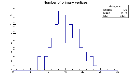
Now we run. Note that it will run over the myoutput.root file that lives in your PhysObjectExtractorTool/PhysObjectExtractor/test area.
./EventLoopAnalysis
This will produce a histograms.root file, which should contain our data_npv histogram. You can open it with ROOT and take a look with the TBrowser:
Key Points
A simple analysis code skeleton can be obtained using ROOT tools
This skeleton can be enhanced to handle a particle physics analysis
Hands-on: Higgs to tau tau Analysis
Overview
Teaching: 0 min
Exercises: 45 minQuestions
What are the main ingredients for a basic Higgs to tau tau analysis
How do I implement more sophisticated selection criteria?
Objectives
Study the event loop implementation of the Higgs to tau tau open data analysis
Lear how to use the ntuples information to perform a particle physics analysis
Disclaimer
During the hands-on sessions, there will be less talking from our side and more reading from yours. You should try to follow the instructions below in detail. If something is not clear, we are here to help. We will try to silently work on the same exercises as you, so we can keep up with possible questions or discussion.
Upgrading the EventLoopAnalysisTemplate
We will try to find Higgses decaying into tau particles in the muon-hadronic channel. We know we need to run the analysis over several datasets (already skimmed with POET) for collisions, background and signal.
Let’s expand our EventLoopAnalysisTemplate.cxx to take care of this. You can download this upgraded file from here. Inside the container or VM, where your skimmed data files reside, you can simply do:
wget https://raw.githubusercontent.com/cms-opendata-workshop/workshop2021-payload-analysisflow/master/EventLoopAnalysisTemplate_upgrade.cxx
Take some time to look at this new file. We have added all the skimmed datasets (which are accessed from the local area) and booked corresponding histograms. We have also taken the opporunity to add more variable into our code (although we are not using most of them yet). If you have a wide screen, you can compare it to the previous version using the sdiff command of similar:
sdiff -w180 -b EventLoopAnalysisTemplate.cxx EventLoopAnalysisTemplate_upgrade.cxx |less
Nos let’s compile it and run:
g++ -std=c++11 -g -O3 -Wall -Wextra -o EventLoopAnalysis EventLoopAnalysisTemplate_upgrade.cxx $(root-config --cflags --libs)
./EventLoopAnalysis
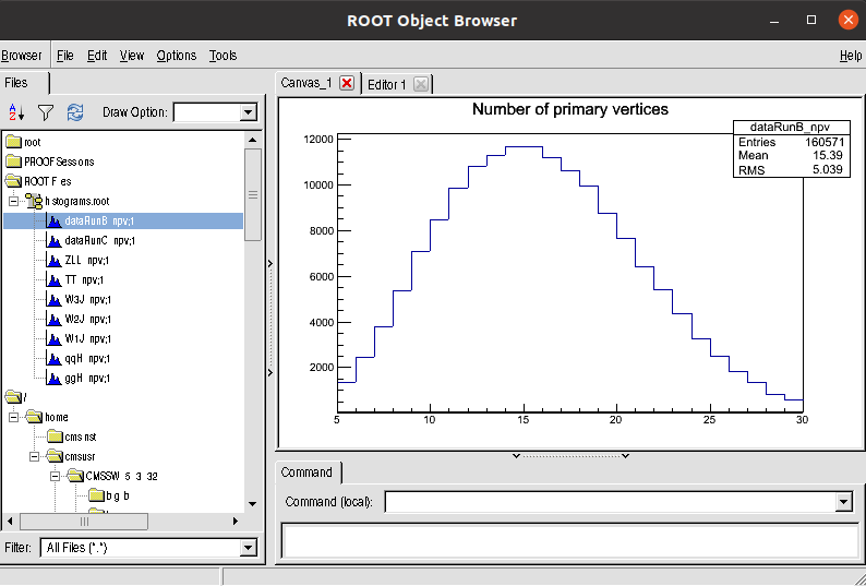
Open the histogram.root file. You will find the npv histogram for all the samples:
EventLoopAnalysis for Higgs to tau tau
Now, as it was our goal, let’s try to implement most of the selection criteria used here and here.
Remember that, at the skimming stage, we already cut rather hard on the requirement to have at least one good muon and at least one good tau. The analysis version of our EventLoopAnalysisTemplate code will, in addition, have:
- A simple selection on the trigger bit that we did not apply earlier
- A cut to select a muon-tau pair from the collections of muons and taus passing the initial selection. The selected pair represents the candidate for this event for a Higgs boson decay to two tau leptons of which one decays to a hadronicfinal state (most likely a combination of pions) and one decays to a muon and a neutrino.
- A muon transverse mass cut for W+jets suppression
Download this code with:
wget https://raw.githubusercontent.com/cms-opendata-workshop/workshop2021-payload-analysisflow/master/EventLoopAnalysis_noiso.cxx
and try to identify the blocks where these selection requirements are applied.
You can compile and run with:
g++ -std=c++11 -g -O3 -Wall -Wextra -o EventLoopAnalysis EventLoopAnalysis_noiso.cxx $(root-config --cflags --libs) -lGenVector
./EventLoopAnalysis
Note the extra flag in the compiler line.
If you check again the histograms file, then you will see that we now have 2 more variables that we will be plotting to try to reproduce the three figures that appear in the original repository.
Muon isolation
However, you are missing one important cut: the requirement that the muon, in the muon-tau pair, is isolated. Based on the original implementation line will you be able to add this cut to our code? Try not to look at the solution too soon and really think about how you will add this cut. (Hint: it is just a single line of code)
solution
The answer is as simple as adding the following after the transverse mass cut:
//Require isolated muon for signal region
 if (!(muon_pfreliso03all->at(idx_1)<0.1)) return;
You can download the final file with:
wget https://raw.githubusercontent.com/cms-opendata-workshop/workshop2021-payload-analysisflow/master/EventLoopAnalysis.cxx
Let’s compile and run once again:
g++ -std=c++11 -g -O3 -Wall -Wextra -o EventLoopAnalysis EventLoopAnalysis.cxx $(root-config --cflags --libs) -lGenVector
./EventLoopAnalysis
If you want you can ispect the histograms.root file.
Making the final plots
One of the reasons why we chose to save the histograms in the way we did was to recycle the plot.py pyROOT script from the original analysis. It needs some touches to make it work in our older version of ROOT, but it is essentially the same. It is mostly a bunch of pyROOT statements to make pretty plots. You could skim through it in order to grasp some understanding of how it works.
You can get a preliminary/compatible version of thi script, plot_nocr.py, with:
wget https://raw.githubusercontent.com/cms-opendata-workshop/workshop2021-payload-analysisflow/master/plot_nocr.py
Now, run it:
python plot_nocr.py
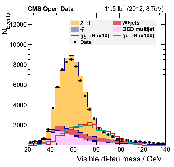
If everything went alright you musta have obtained these figures:
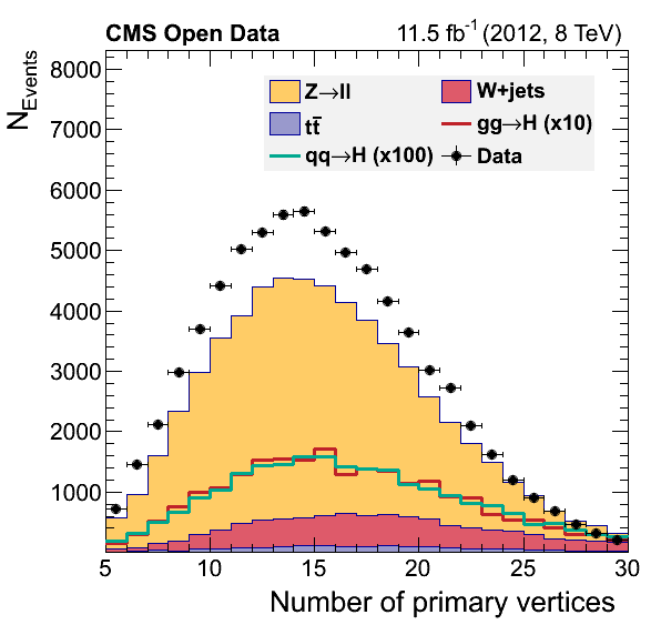
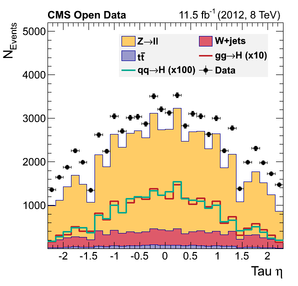
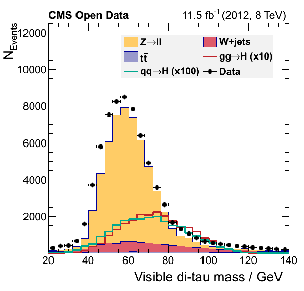
What happened?
Did we discover something? Or did we forget some background process? You will try to fix this during the offline challenge.
Key Points
The Higgs to tau tau simplified analysis can be implemente in an event loop style
There is some problem with our final plots, but we shal fix that ….
Break
Overview
Teaching: 0 min
Exercises: 15 minQuestions
Objectives
Finally a break of 15’ before the beginning of the Cloud Computing lesson…. We will see you there
Key Points
Offline Challenge: Data-driven QCD estimation
Overview
Teaching: 0 min
Exercises: 60 minQuestions
Is it possible to estimate the QCD contribution from data?
Objectives
Implement a simple data-driven method for QCD estimation
Data-driven QCD estimation
These comments in the original plot.py script, assert the possibility of estimating the QCD contribution in our analysis.
To give you a head-start, this version of the plot.py will work with the output of the final version of our EventLoopAnalysis.cxx code. Your task consists of modifying the latter code so we can complete the final plots by adding the QCD background.
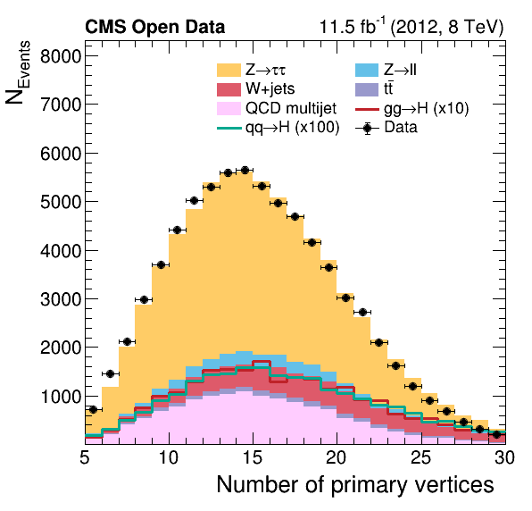
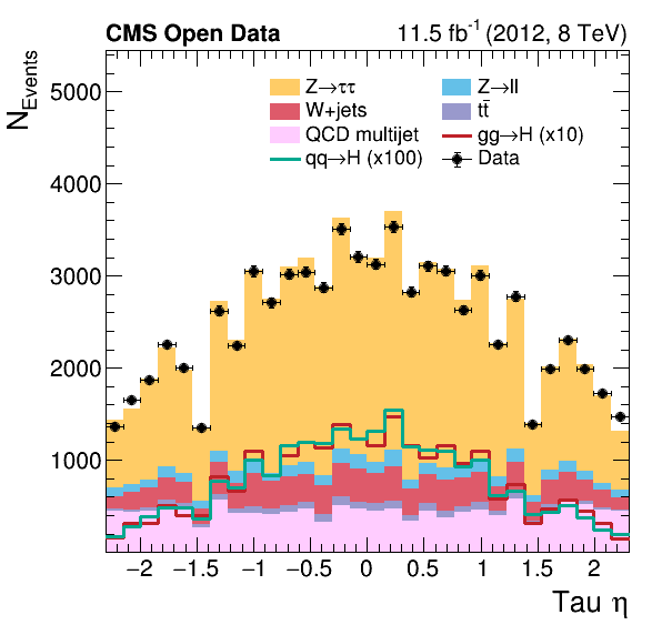
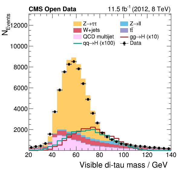
Final plots should look like:
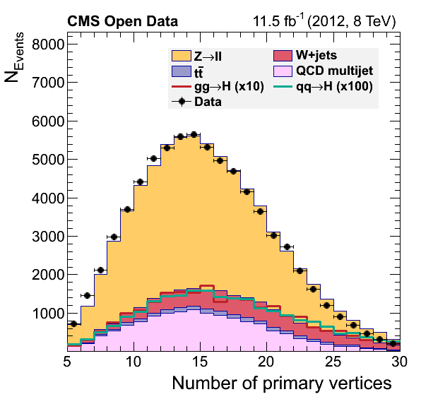
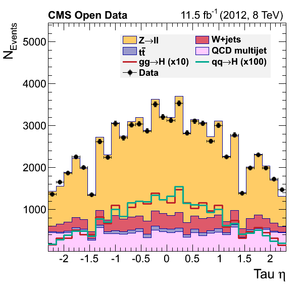
Key Points
The QCD multijet background can be estimated using a data-driven approach
Solution and discussion
Overview
Teaching: 0 min
Exercises: 40 minQuestions
Where you able to find a way of implementing the data-driven QCD contribution?
Did you notice anything different in our plots compared to the original ones?
Objectives
Show the solution to yesterday’s QCD estimation challenge
Discuss about the analysis features and possible limitations
The solution
Here is the solution to yesterday’s adventure. Let’s go through it.
The difference in our plots
Did you notice a difference between our final plots below and the ones from our reference? What would it take to make a closer replica?
|
 |
|---|
|
 |
|---|
|
 |
|---|
Key Points
The Higgs to tau tau simplified analysis offers a great opportunity to learn about the most basic ingredients in an analysis flow