Content from Introduction
Last updated on 2024-07-09 | Edit this page
Estimated time: 10 minutes
Overview
Questions
- What is the point of these exercises?
- How do I find the data I want to work with?
Objectives
- To understand why we start with the Open Data Portal
- To understand the basics of how the datasets are divided up
Ready to go?
The first part of this lesson is done entirely in the browser.
Then, Episode 4:
How to access metadata on the command line? requires the use of a
command-line tool. It is available as a Docker container or it can be
installed with pip. Make sure you have completed the Docker
pre-exercise and have docker installed.
Episode 5: What is in the data? is done in the root or python tools container. Make sure you have these containers available.
You’ve got a great idea! What’s next?
Suppose you have a great idea that you want to test out with real data! You’re going to want to know:
-
This may mean
- finding simulated physics processes that are background to your signal
- finding simulated physics processes for your signal, if they exist
- possibly just finding simulated datasets where you know the answer, allowing you to test your new analysis techniques.
In this lesson, we’ll walk through the process of finding out what data and Monte Carlo are available to you, how to find them, and how to examine what data are in the individual data files.
What is a Monte Carlo dataset?
You’ll often hear about physicists using Monte Carlo data or sometimes just referring to Monte Carlo. In both cases, we are referring to simulations of different physics processes, which then mimics how the particles would move through the CMS detector and how they might be affected (on average) as they pass through the material. This data is then processed just like the “real” data (referred to as collider data).
In this way, the analysts can see how the detector records different physics processes and best understand how these processes “look” when we analyze the data. This better helps us understand both the signal that we are looking for and the backgrounds which might hide what we are looking for.
First of all, let’s understand how the data are stored and why we need certain tools to access them.
The CERN Open Data Portal
In some of the earliest discussions about making HEP data publicly available there were many concerns about people using and analyzing “other people’s” data. The concern centered around well-meaning scientists improperly analyzing data and coming up with incorrect conclusions.
While no system is perfect, one way to guard against this is to only release well-understood, well-calibrated datasets and to make sure open data analysts only use these datasets. These datasets are given a Digital Object Identifier (DOI) code for tracking. And if there are ever questions about the validity of the data, it allows us to check the data provenance.
DOI
The Digital Object Identifier (DOI) system allows people to assign a unique ID to any piece of digital media: a book, a piece of music, a software package, or a dataset. If you want to learn more about the DOI process, you can learn more at their FAQ.
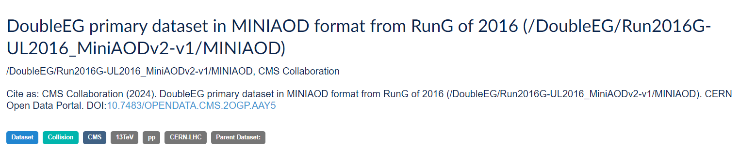
Challenge!
You will find that all the datasets have their DOI listed at the top of their page on the portal. Can you locate where the DOI is shown for this dataset, Record 30521, DoubleEG primary dataset in NANOAOD format from RunG of 2016 (/DoubleEG/Run2016G-UL2016_MiniAODv2_NanoAODv9-v1/NANOAOD)
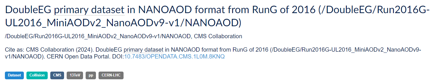
With a DOI, you can create citations to any of these records, for example using a tool like doi2bib.
Provenance
You will hear experimentalists refer to the “provenance” of a dataset. From the Cambridge dictionary, provenance refers to “the place of origin of something”. The way we use it, we are referring to how we keep track of the history of how a dataset was processed: what version of the software was used for reconstruction, what period of calibrations was used during that processing, etc. In this way, we are documenting the data lineage of our datasets.
From Wikipedia
Data lineage includes the data origin, what happens to it and where it moves over time. Data lineage gives visibility while greatly simplifying the ability to trace errors back to the root cause in a data analytics process.
Provenance is an an important part of our data quality checks and another reason we want to make sure you are using only vetted and calibrated data.
This lesson
For all the reasons given above, we encourage you to familiarize yourself with the search features and options on the portal. With your feedback, we can also work to create better search tools/options and landing points.
This exercise will guide you through the current approach to finding data and Monte Carlo. Let’s go!
Key Points
- Finding the data is non-trivial, but all the information is on the portal
- A careful understanding of the search options can help with finding what you need
Content from Where are the datasets?
Last updated on 2024-06-27 | Edit this page
Estimated time: 10 minutes
Overview
Questions
- Where do I find datasets for data and Monte Carlo?
Objectives
- Be able to find the data and Monte Carlo datasets
CERN Open Data Portal
Our starting point is the landing page for CERN Open Data Portal. You should definitely take some time to explore it. But for now we will select the CMS data.
CERN Open Data Portal
The landing page for the CERN Open
Data Portal. 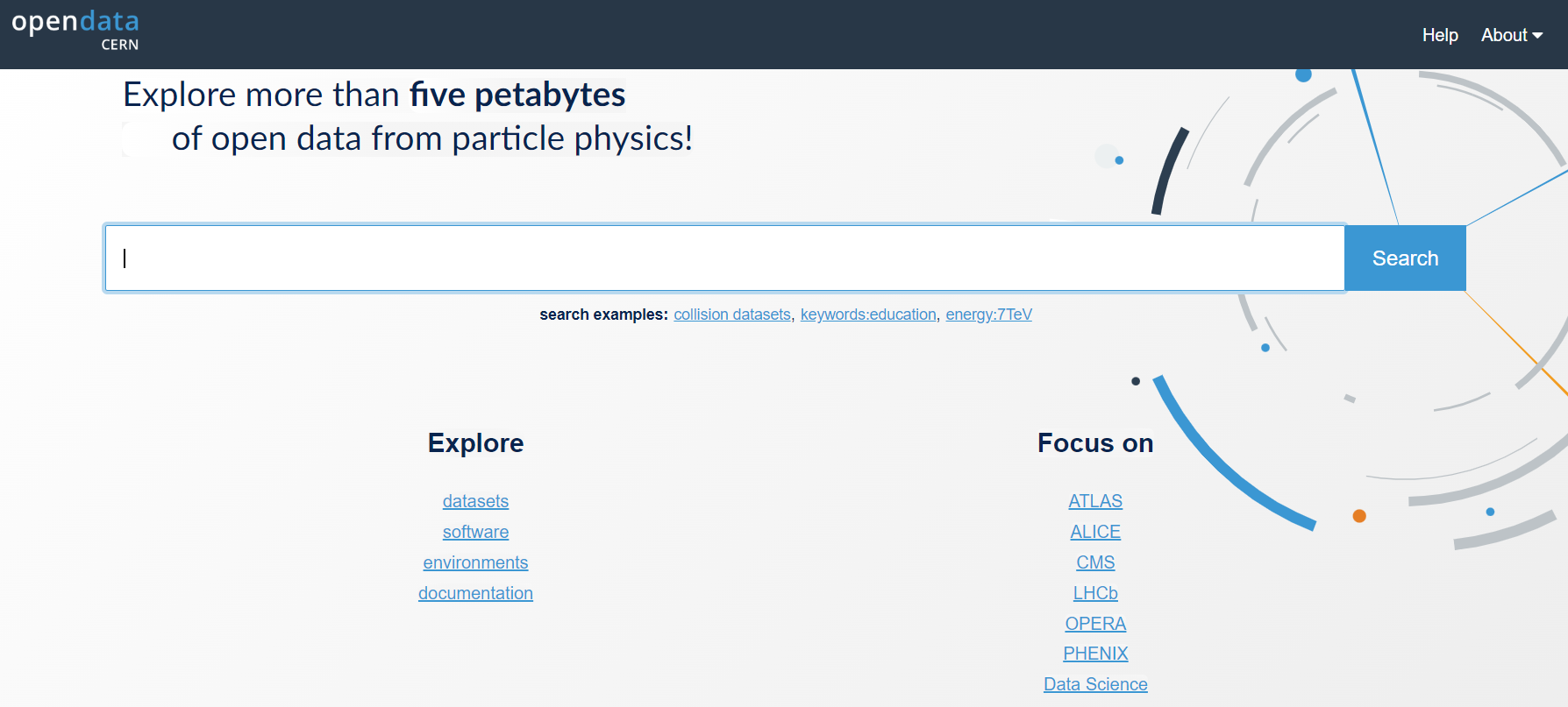
Make a selection!
Find the CMS link under Focus on and click on it.
CMS-specific datasets
The figure below shows the website after we have chosen the CMS data. Note the left-hand sidebar that allows us to filter our selections. Let’s see what’s there.
CERN Open Data Portal - CMS data
The first pass to filter on CMS data 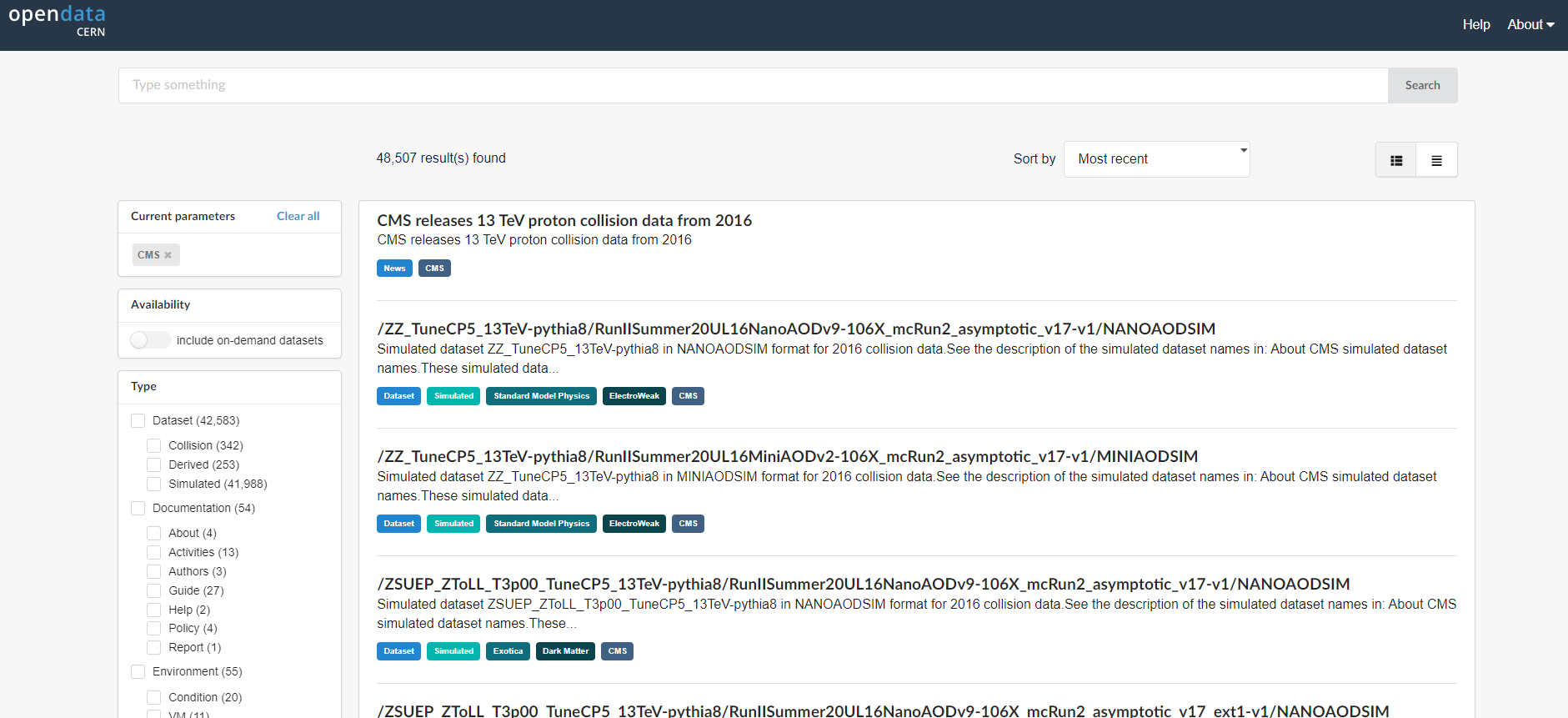
At first glance we can see a few things. First, there is an option to select only Dataset rather than documentation or software or similar materials. Great! Going forward we’ll select Dataset.
Next, scrolling down to see the search options in the left bar, we see that there are a lot of entries for data from 2010, 2011, 2012, 2015, and 2016, the 7 TeV, 8 TeV and 13 TeV running periods. We’ll be working with 2016 data for these exercises.
Make a selection!
For the next episode, let’s select Dataset and 2016.
Key Points
- Use the filter selections in the left-hand sidebar of the CERN Open Data Portal to find datasets.
Content from What data and Monte Carlo are available?
Last updated on 2024-07-02 | Edit this page
Estimated time: 15 minutes
Overview
Questions
- What data and run periods are available?
- What data do the collision datasets contain?
- What Monte Carlo samples are available?
Objectives
- To be able to navigate the CERN Open Data Portal’s search tools
- To be able to find what collision data and Monte Carlo datasets there are using these search tools
Data and run periods
We make a distinction between data which come from the real-life CMS detector and simulated Monte Carlo data. In general, when we say data, we mean the real, CMS-detector-created data.
The data available are from what is known as Run 1, spanning 2010-2012, and Run 2 spanning 2015-2018. The latest data are from 2016 and were release in April 2024. The run periods each year can also be broken into A, B, C, and so-on, sub-periods and you may see that in some of the dataset names.
Make a selection!
If you are coming from the previous page you should have selected CMS, Dataset, and 2016.
CERN Open Data Portal - CMS datasets
Selecting CMS, Dataset, and 2016.
Your view might look slightly different than this screenshot as the available datasets and tools are regularly updated.
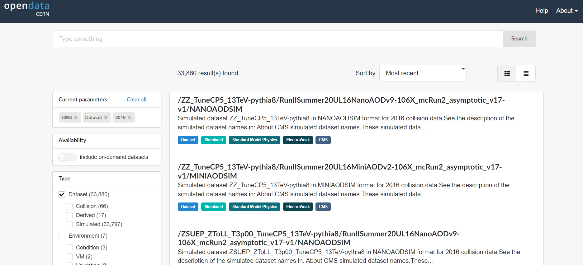
When Dataset is selected, there are 3 subcategories:
- Collision refers to the real data that came off of the CMS detector.
- Derived refers to datasets that have been further processed for some specific purpose, such as outreach and education or the ispy event display.
- Simulated refers to Monte Carlo datasets.
Make a selection!
Let’s now select uniquely the Collision option under Dataset.
Collision data
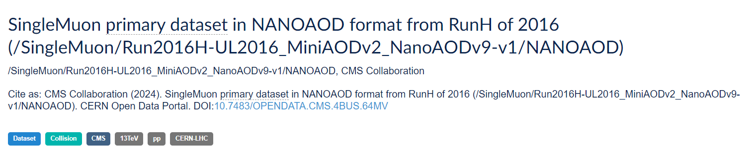
When you select Collision you’ll see a lot of datasets with names that may be confusing. Let’s take a look at two of them and see if we can break down these names.
CERN Open Data Portal - Sample CMS collision datasets
There are three (3) parts to the names, separated by
/.
Dataset name
DoubleEG or SingleMuon is the name of the dataset. Events stored in these primary datasets were selected by triggers of usually of a same type. For each dataset, the list of triggers is listed in the dataset record. You can learn more about them in the lesson of the CMS Open Data workshops, but for now, remind yourself that they select out some subset of the collisions based on certain criteria in the hardware or software.
Some of the dataset names are quite difficult to intuit what they mean. Others should be roughly understandable. For example,
- DoubleEG contains mainly events with at least two electrons (E) or photons (G: gamma) above a certain energy threshold.
- SingleMu contains mainly events with at least one muon above a certain momentum threshold.
- MinimumBias events are taken without any trigger or selection criteria.
Run period and processing string
Run2016G and Run2016H refer to when the data were taken, and UL2016_MiniAODv2-v1 and UL2016_MiniAODv2_NanoAODv9-v1 when and how the data were reprocessed. The details are not so important for you because CMS only releases vetted data. If you were a CMS analyst working on the data as it was being processed, you might have to shift your analysis to a different dataset once all calibrations were completed.
Data format
CMS data are stored in different formats:
- RAW files contain information directly from the detector in the form of hits from the TDCs/ADCs. (TDC refers to to Time to Digital Converter and ADC refers to to Analog to Digital Converter. Both of these are pieces of electronics which convert signals from the components of the CMS detector to digital signals which are then stored for later analysis.) These files are not a focus of this workshop.
- AOD stands for Analysis Object Data. This was the first stage of data where analysts can really start physics analysis when using Run 1 data.
- MINIAOD is a slimmer format of AOD, in use in CMS from Run 2 data on.
- NANOAOD is slimmed-down version of MINIAOD, and, in contrast to all other formats above, does not require CMS-specific software for analysis.
Further information
If you click on the link to any of these datasets, you will find even more information, including
- The size of the dataset
- Information on the what is the recommended software release to analyze this dataset
- Information on the available software containers
- How were the data selected including the details of the trigger selection criteria.
- Validation information
- A list of all the individual ROOT files in which this dataset is stored
There are multiple text files that contain the paths to these ROOT files. If we click on any one of them, we see something like this.
CERN Open Data Portal - CMS dataset file isting
Sample listing of some of the ROOT files in the /SingleMuon/Run2016H-UL2016_MiniAODv2_NanoAODv9-v1/NANOAOD dataset.
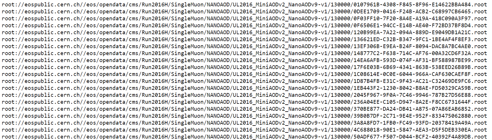
The prepended root: is because of how these files are
accessed. We’ll use these directory paths when we go to inspect some of
these files. The grouping of the files in separate lists comes from the
reprocessing computing operations and has no particular meaning.
Monte Carlo
We can go through a similar exercise with the Monte Carlo data. One major difference is that the Monte Carlo are not broken up by trigger. Instead, when you analyze the Monte Carlo, you will apply the trigger to the data to simulate what happens in the real data.
For now, let’s look at some of the Monte Carlo datasets that are available to you.
Make some selections! But first make some unselections!
Unselect everything except for 2016, CMS, Dataset, and then select Simulated (under Dataset).
Scroll down to see the options under Category in the left bar.
CERN Open Data Portal - CMS Monte Carlo datasets
Monte Carlo dataset category search options
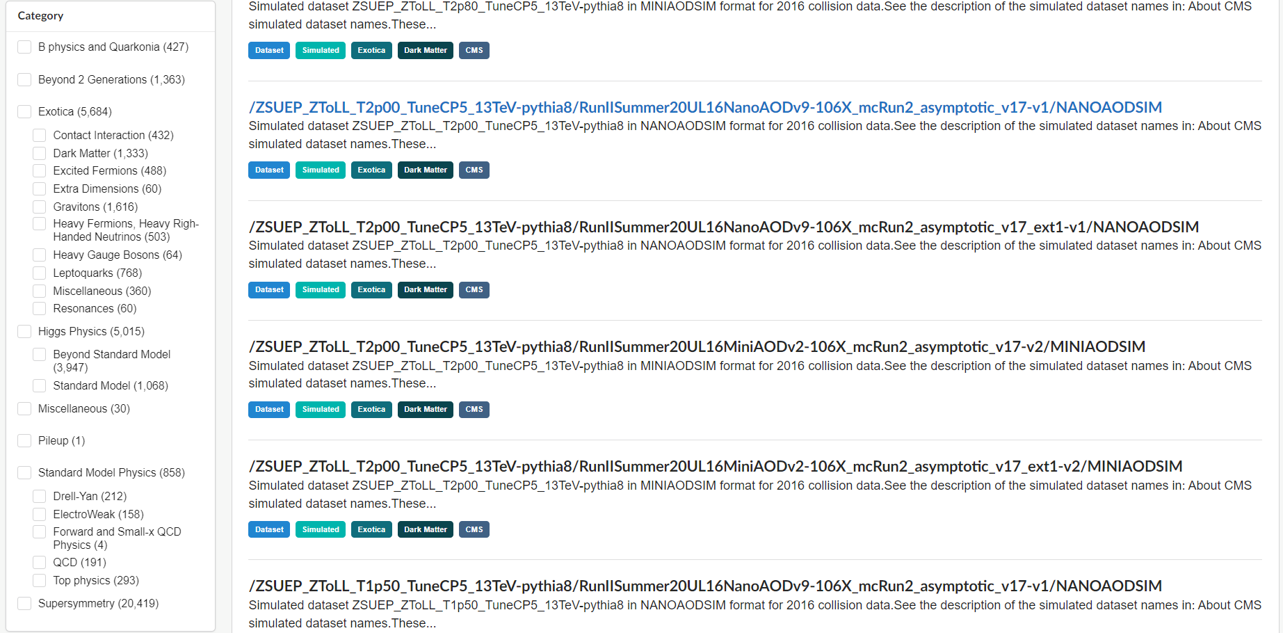
There are a lot of Monte Carlo samples! It’s up to you to determine which ones might contribute to your analysis. The names try to give you some sense of the primary process, subsequent decays, the collision energy and specific simulation software (e.g. Pythia), but if you have questions, reach out to the organizers.
As with the collision data, here are three (3) parts to the names,
separated by /.
Let’s look at one of them: /DYToMuMu_M-120To200_TuneCP5_13TeV-powheg-pythia8/RunIISummer20UL16NanoAODv9-106X_mcRun2_asymptotic_v17-v1/NANOAODSIM
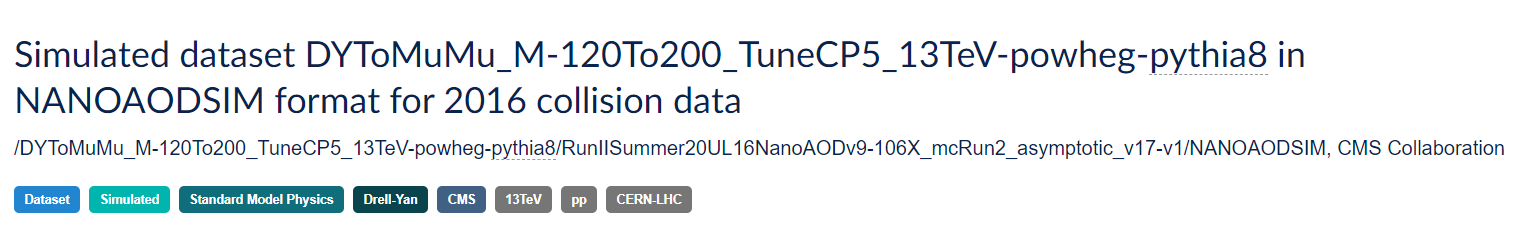
Physics process/Monte Carlo sample
DYToMuMu_M-120To200_TuneCP5_13TeV-powheg-pythia8 is hard to understand at first glance, but if we take our time we might be able to intuit some of the meaning. This appears to simulate a Drell-Yan process in which two quarks interact to produce a virtual photon/Z boson which then couples to two leptons. The M-120To200 refers to a selection that has been imposed requiring the mass of the di-lepton pair to be between 120 and 200 50 GeV/c^2. TuneCP5 refers to the the set of CMS underlying-event parameters of PYTHIA8 event generator. 13TeV is the center-of-mass energy of the collision used in the simulation, the remaining fields tell us what software was used to generate this (powheg for event generation and pythia8 for hadronization).
Processing and Global tag
RunIISummer20UL16NanoAODv9-106X_mcRun2_asymptotic_v17-v1 refers to how and when this Monte Carlo was processed. The details are not so important for you because the open data coordinators have taken care to only post vetted data. But it is all part of the data provenance.
Data format
The last field refers to the data format and here again there is a slight difference.
- MINIAODSIM or NANOAODSIM stands for Mini or Nano Analysis Object Data - Simulation. This is the same as the MINIAOD or NANOAOD format used in the collision data, except that there are some extra fields that store information about the original, generated 4-vectors at the parton level, as well as some other Monte Carlo-specific information.
One difference is that you will want to select the Monte Carlo events that pass certain triggers at the time of your analysis, while that selection was already done in the data by the detector hardware/software itself.
If you click on any of these fields, you can see more details about the samples, similar to the collision data.
More Monte Carlo samples
If you would like a general idea of what other physics processes have been simulated, you can check scroll down the sidebar until you come to Category.
Challenge: find generator parameters
Select some Monte Carlo datasets and see if you can find the generator information in the dataset provenance.
You may have to do a bit of poking around to find the dataset that is most appropriate for what you want to do, but remember, you can always reach out to the organizers.
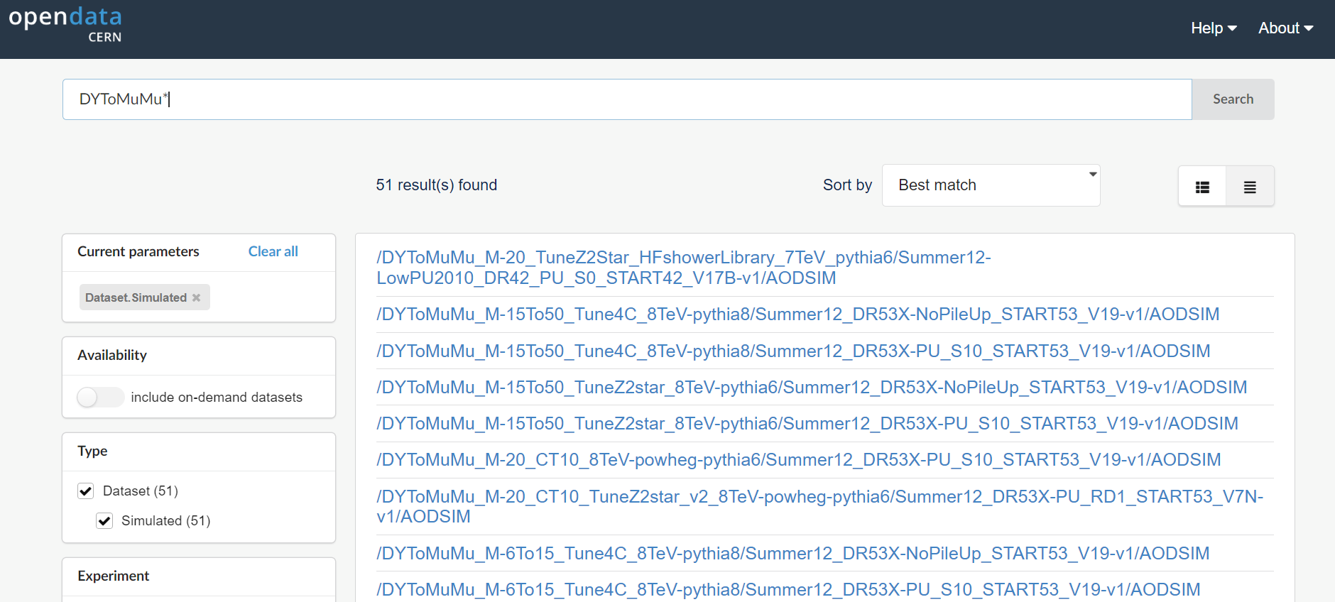
Search tips
The category search is helpful to find relevant Monte Carlo datasets, but that’s not enough! The most recent CMS data release includes more than 40000 Monte Carlo datasets and even split into smaller categories, your category of interest might have several hundred entries.
A help page provides some search tips and some more here:
For 2016 data, you can select the format that you are going to use and that will half the number of entries. Choose, for example nanoaodsim under File type.
To fit more entries to one page, you can choose the list view from the search, and increase the number of results per page. It will make the search slower.
To search a string in the record title use, for example:
GluGluHToGG*DYToMuMu**sherpa**flat*
Callout
Always check the generator parameters from the dataset provenance to be sure what you get!
Key Points
- The collision data are directed to different datasets based on trigger decisions.
- The Monte Carlo datasets contain a specific simulated physics process.
Content from How to access metadata on the command line?
Last updated on 2024-07-02 | Edit this page
Estimated time: 15 minutes
Overview
Questions
- What is cernopendata-client?
- How to use cernopendata-client container image?
- How to get the list of files in a dataset on the command line?
Objectives
- To be able to access the information programmatically
Dataset information
Each CMS Open Data dataset comes with metadata that describes its contents (size, number of files, number of events, file listings, etc) and provenance (data-taking or generator configurations, and information on reprocessings), or provides usage instructions (the recommended CMSSW version, Global tag, container image, etc). The previous section showed how this information is displayed on the CERN Open Data portal. Now we see how it can also be retrieved programmatically or on the command line.
Command-line tool
cernopendata-client
is a command-line tool to download files or metadata of CERN Open Data
portal records. It can be installed
with pip or used through the container image.
As you already have Docker installed, we use the latter option. Pull the container image with:
Display the command help with:
OUTPUT
Usage: cernopendata-client [OPTIONS] COMMAND [ARGS]...

  Command-line client for interacting with CERN Open Data portal.

Options:
  --help  Show this message and exit.

Commands:
  download-files      Download data files belonging to a record.
  get-file-locations  Get a list of data file locations of a record.
  get-metadata        Get metadata content of a record.
  list-directory      List contents of a EOSPUBLIC Open Data directory.
  verify-files        Verify downloaded data file integrity.
  version             Return cernopendata-client version.
This is equivalent to running
cernopendata-client --help, when the tool is installed with
pip. The command runs in the container, it displays the
output and exits. Note the flag --rm: it removes the
container created by the command so that they are not accumulated in
your container list each time you run a command.
Get dataset information
Each dataset has a unique identifier, a record id (or
recid), that shows in the dataset URL and can be used in
the cernopendata-client commands. For example, in the previous sections,
you have seen that file listings are in multiple text files. To get the
list of all files in the /SingleMuon/Run2016H-UL2016_MiniAODv2_NanoAODv9-v1/NANOAOD
dataset, use the following (recid of this dataset is
30563):
BASH
docker run -i -t --rm docker.io/cernopendata/cernopendata-client get-file-locations --recid 30563 --protocol xrootdor pipe it to a local file with:
BASH
docker run -i -t --rm docker.io/cernopendata/cernopendata-client get-file-locations --recid 30563 --protocol xrootd > files-recid-30563.txtExplore other metadata fields
Summary
cernopendata-client is a handy tool for getting dataset
information programmatically in scripts and workflows.
We will be working on getting all metadata needed for an analysis of CMS Open Data datasets retrievable through cernopendata-client, and some improvements are about to be included in the latest version. Let us know what you would like to see implemented!
Key Points
- cernopendata-client is a command-line tool to download dataset files and metadata from the CERN Open Data portal.
Content from What is in the datafiles?
Last updated on 2024-07-08 | Edit this page
Estimated time: 10 minutes
Overview
Questions
- How do I inspect these files to see what is in them?
Objectives
- To be able to see what objects are in the data files
In the following, we will learn about CMS data in the NANOAOD format. This is the data format that can be accessed without CMS-specific software using ROOT or python tools.
NANOAOD variable list
Each NANOAOD dataset has the variable list with a brief description attached to the portal record. You will learn more about the variables for different types of physics objects in the Physics Objects lesson
Challenge: variables
Find the variable listings for a collision data record and a Monte Carlo data record. What are the differences? What is the same?
The data records have a “Luminosity” block with some beam related information whereas MC records have a “Runs” block with event generation information.
The MC records have event generator or simulation information in the “Events” block.
The variables of reconstructed objects, such as Muons, are the same for data and MC.
Inspect datasets with ROOT
This part of the lesson will be done from within the ROOT tools container. You should have it available, start it with:
All ROOT commands will be typed inside that environment.
If you are using VNC for the graphics, remember to start it before starting ROOT in the container prompt:
Work through the quick introduction to getting started with CMS NANOAOD Open Data in the getting started guide page on the CERN Open Data portal.
You will learn:
Inspect datasets with python tools
This part of the lesson will be done from within the python tools container. You should have it available, start it with:
Start the jupyter lab with
Open a new jupyter notebook from the jupyter lab tab that the container will open in your browser. Type the commands in code cells of the notebook.
First, import some python libraries:
- uproot is a python inteface to ROOT
- matplotlib can be used for plotting
- numpy is a python package for scientific computing
- awkard is a python library for variable-size data
Then, open a file from a dataset:
PYTHON
file = uproot.open("root://eospublic.cern.ch//eos/opendata/cms/Run2016H/SingleMuon/NANOAOD/UL2016_MiniAODv2_NanoAODv9-v1/120000/61FC1E38-F75C-6B44-AD19-A9894155874E.root")Print out event content with python tools
You can check the content blocks of the file with
OUTPUT
{'tag;1': 'TObjString',
 'Events;1': 'TTree',
 'LuminosityBlocks;1': 'TTree',
 'Runs;1': 'TTree',
 'MetaData;1': 'TTree',
 'ParameterSets;1': 'TTree'}
Events is the TTreeobject that contains the
variables of interest to us. Get it from the data with:
You can list the full list of variables with
Now, fetch some variables of interest, e.g. take all muon pt values in an array
Challenge: inspect pt
Find out the type of the pt array. Print values of some of its elements. What do you observe?
Find the type with
OUTPUT
awkward.highlevel.ArrayPrint out some of the values with
OUTPUT
[[23.1], [39.3], [24.1], [91.9, 52.7], ... [88.7, 14.2], [58.9], [27.1], [50]]Note that the muon pt array can contain one or more elements, depending on the number of reconstructed muons in the event.
From the awkward array documentation, you can find out hot to choose the events with exactly two reconstructed muons:
OUTPUT
<Array [[91.9, 52.7], ... [88.7, 14.2]] type='2713 * var * float32'>You can learn about awkward arrays and much more in the HEP Software Foundation Scikit-HEP tutorial.
Plot a variable with python tools
Common python plotting tools cannot handle arrays or arrays with different sizes, such as the muon pt. If you want to plot all muon pts, “flatten” the pt array first:
Now plot the muon pt values with
You could also plot directly ptflat variable, but it you
want to introduce some cuts that need the knowledge that certain values
belong to the same event, you need to do them to the original pt array.
For example, plotting the events with 2 muons:
PYTHON
plt.hist(ak.flatten(pt),bins=200,range=(0,200))
plt.hist(ak.flatten(pt[ak.num(pt) == 2]),bins=200,range=(0,200))
plt.show()
This is what you will see:
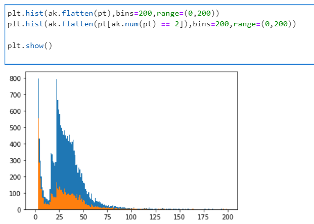
If you’ve chosen another dataset or another file, it will look different.
Homework: complete the homework form!
Please visit the assignment form and answer some questions about navigating the Open Data Portal to find Open Data. You need to sign in and click on the submit button in order to save your work. You can go back to edit the form at any time.
Key Points
- It’s useful to inspect the files before diving into the full analysis.
- Some files may not have the information you’re looking for.