Physics Object Extractor Tool
Overview
Teaching: 10 min
Exercises: minQuestions
What are the main CMS Physics Objects and how do I access them?
Objectives
Identify CMS physics objects
Identify object code collections in AOD files
Access an object code collection
Learn member functions for standard momentum-energy vectors
CMS uses the phrase “physics objects” to speak broadly about particles that can be identified via signals from the CMS detector. A physics object typically began as a single particle, but may have showered into many particles as it traversed the detector. The principle physics objects are:
- muons
- electrons
- taus
- photons
- jets
- missing transverse momentum
Viewing modules in a data file
CMS AOD files store all physics objects of the same type in “modules”. These modules are
data structures that act as containers for multiple instances of the same C++ class. The edmDumpEventContent command
show below lists all the modules in a file. As an example,
the “muons” module in AOD contains many reco::Muon objects (one per muon in the event).
$ edmDumpEventContent root://eospublic.cern.ch//eos/opendata/cms/MonteCarlo2012/Summer12_DR53X/TTbar_8TeV-Madspin_aMCatNLO-herwig/AODSIM/PU_S10_START53_V19-v2/00000/000A9D3F-CE4C-E311-84F8-001E673969D2.root
Type                                  Module                      Label             Process
----------------------------------------------------------------------------------------------
...
vector<reco::Muon>                    "muons"                     ""                "RECO"
vector<reco::Muon>                    "muonsFromCosmics"          ""                "RECO"
vector<reco::Muon>                    "muonsFromCosmics1Leg"      ""                "RECO"
...
vector<reco::Track>                   "cosmicMuons"               ""                "RECO"
vector<reco::Track>                   "cosmicMuons1Leg"           ""                "RECO"
vector<reco::Track>                   "globalCosmicMuons"         ""                "RECO"
vector<reco::Track>                   "globalCosmicMuons1Leg"     ""                "RECO"
vector<reco::Track>                   "globalMuons"               ""                "RECO"
vector<reco::Track>                   "refittedStandAloneMuons"   ""                "RECO"
vector<reco::Track>                   "standAloneMuons"           ""                "RECO"
vector<reco::Track>                   "refittedStandAloneMuons"   "UpdatedAtVtx"    "RECO"
vector<reco::Track>                   "standAloneMuons"           "UpdatedAtVtx"    "RECO"
vector<reco::Track>                   "tevMuons"                  "default"         "RECO"
vector<reco::Track>                   "tevMuons"                  "dyt"             "RECO"
vector<reco::Track>                   "tevMuons"                  "firstHit"        "RECO"
vector<reco::Track>                   "tevMuons"                  "picky"           "RECO"
Note that this file also contains many other muon-related modules: two modules of reco::Muon muons
from cosmic-ray events, and many modules of reco::Track objects that give lower-level tracking
information for muons. As you can see, the AOD file contains MANY modules, and not all of them are related directly to
physics objects. Other important modules might include:
- Tracks and vertices
- Calorimeter clusters and other detector information
- Particle Flow candidates
- Triggers
- Pileup (info about multiple collisions from the same pp crossing)
- Generator-level information (in simulation)
Physics Object Extractor Tool (POET)
Setup
The PhysObjectExtractorTool (POET) repository is the example we will use for accessing information from AOD files. If you have not already done so, please check out this repository:
$ cd ~/CMSSW_5_3_32/src/
$ cmsenv
$ git clone git://github.com/cms-legacydata-analyses/PhysObjectExtractorTool.git
$ cd PhysObjectExtractorTool
$ scram b
In the various source code files for this tool, found in PhysObjectExtractor/src/, the definitions of different classes are included. Continuing with muons as the example, we include the following in PhysObjectExtractor/src/MuonAnalyzer.cc:
#include "DataFormats/MuonReco/interface/Muon.h"
#include "DataFormats/MuonReco/interface/MuonFwd.h"
#include "DataFormats/MuonReco/interface/MuonSelectors.h"
You learned about the EDAnalyzer class in the pre-exercises. The POET is an EDAnalyzer – let’s refresh how to access data inside the EDAnalyzer. The “analyze” function of an EDAnalyzer is performed once per event. Muons can be accessed like this:
void
MuonAnalyzer::analyze(const edm::Event &iEvent, const edm::EventSetup &iSetup)
{

  using namespace edm;
  using namespace std;

  Handle<reco::MuonCollection> mymuons;
  iEvent.getByLabel(muonInput, mymuons); // muonInput opens "muons"
The result of the getByLabel command is a variable called “mymuons” which is a collection of all the muon objects.
Collection classes are generally constructed as std::vectors. We can
quickly access create a loop to access individual muons:
for (reco::MuonCollection::const_iterator itmuon=mymuons->begin(); itmuon!=mymuons->end(); ++itmuon){
    if (itmuon->pt() > mu_min_pt) {
        // do things here, see below!
    }
}
Accessing basic kinematic quantities
Many of the most important kinematic quantities defining a physics object are accessed in a common way across all the objects. All objects have associated energy-momentum vectors, typically constructed using transverse momentum, pseudorapdity, azimuthal angle, and mass or energy.
In MuonAnalyzer.cc the muon four-vector elements are accessed as shown below. The
values for each muon are stored into an array, which will become a branch in a ROOT TTree.
for (reco::MuonCollection::const_iterator itmuon=mymuons->begin(); itmuon!=mymuons->end(); ++itmuon){
  if (itmuon->pt() > mu_min_pt) {

    muon_e.push_back(itmuon->energy());
    muon_pt.push_back(itmuon->pt());
    muon_eta.push_back(itmuon->eta());
    muon_phi.push_back(itmuon->phi());

    muon_px.push_back(itmuon->px());
    muon_py.push_back(itmuon->py());
    muon_pz.push_back(itmuon->pz());

    muon_mass.push_back(itmuon->mass());

}
You will see the same type of kinetmatic member functions in all the different analyzers in the src/ folder!
The POET configuration file
As you learned in the pre-exercise, EDAnalyzers can be configured using a python file. In POET this is called python/poet_cfg.py.
It contains all of the processing setup as well as configuration for each EDAnalyzer we can run. The first several analyzers are configured here:
#---- Configure the PhysObjectExtractor modules!

#---- More information about InputCollections at https://twiki.cern.ch/twiki/bin/view/CMSPublic/SWGuideRecoDataTable
process.myevents = cms.EDAnalyzer('EventAnalyzer')

process.myelectrons = cms.EDAnalyzer('ElectronAnalyzer',
         InputCollection = cms.InputTag("gsfElectrons")
         )

process.mymuons = cms.EDAnalyzer('MuonAnalyzer',
     InputCollection = cms.InputTag("muons")
     )

process.myphotons = cms.EDAnalyzer('PhotonAnalyzer',
                                   InputCollection = cms.InputTag("photons")
       )
If multiple collections exist with the same name in the “Module” column from edmDumpEventContent, more specific names from the “Label” and “Process” columns can be specified using colon separators: cms.InputTag("module:label:process")
Running POET requires 2 command-line arguments:
isData: true for data and false (default) for simulation,doPat: true to use the Physics Analysis Toolkit for jets and met (more on that later!) or false (default) to run without this.
$ cmsRun python/poet_cfg.py False True # run in PAT mode on simulation
Key Points
CMS physics objects include: muons, electrons, taus, photons, and jets.
Missing transverse momentum is derived from physics objects (negative vector sum).
Objects are stored in separate collections in the AOD files
Objects can be accessed one-by-one via a for loop
Physics objects in CMS inherit common member functions for the 4-vector quantities of transverse momentum, polar/azimuthal angles, and mass/energy.
Electrons and Photons
Overview
Teaching: 10 min
Exercises: 0 minQuestions
How are electrons and photons treated in CMS OpenData?
Objectives
Learn electron member functions for common track-based quantities
Bookmark informational web pages for electrons and photons
Learn member functions for identification and isolation of electrons
Learn member functions for electron detector-related quantities
Electrons and photons are both reconstructed in the electromagnetic calorimeter in CMS, so they share many common properties and functions.
In POET we will study the ElecronAnalyzer.cc and PhotonAnalyzer.cc.
Electron 4-vector and track information
In the loop over the electron collection in ElectronAnalyzer.cc, we access elements of the four-vector as shown in the last episode:
for (reco::GsfElectronCollection::const_iterator itElec=myelectrons->begin(); itElec!=myelectrons->end(); ++itElec){
    ...
    electron_e.push_back(itElec->energy());
    electron_pt.push_back(itElec->pt());
    ...
}
Most charged physics objects are also connected to tracks from the CMS tracking detectors. The charge of the object can be queried directly:
electron_ch.push_back(itElec->charge());
Information from tracks provides other kinematic quantities that are common to multiple types of objects.
Often, the most pertinent information about an object to access from its
associated track is its impact parameter with respect to the primary interaction vertex.
Since muons can also be tracked through the muon detectors, we first check if the track is
well-defined, and then access impact parameters in the xy-plane (dxy or d0) and along
the beam axis (dz), as well as their respective uncertainties.
math::XYZPoint pv(vertices->begin()->position());  // line 148
...

auto trk = itElec->gsfTrack();
...
electron_dxy.push_back(trk->dxy(pv));
electron_dz.push_back(trk->dz(pv));
electron_dxyError.push_back(trk->d0Error());
electron_dzError.push_back(trk->dzError());
Photons, as neutral objects, do not have a direct track link (though displaced track segments may appear from electrons or positrons produced by the photon as it transits the detector material). While the charge() method exists for all objects, it is not used in photon analyses.
Detector information for identification
The most signicant difference between a list of certain particles from a Monte Carlo generator and a list of the corresponding physics objects from CMS is likely the inherent uncertainty in the reconstruction. Selection of “a muon” or “an electron” for analysis requires algorithms designed to separate “real” objects from “fakes”. These are called identification algorithms.
Other algorithms are designed to measure the amount of energy deposited near the object, to determine if it was likely produced near the primary interaction (typically little nearby energy), or from the decay of a longer-lived particle (typically a lot of nearby energy). These are called isolation algorithms. Many types of isolation algorithms exist to deal with unique physics cases!
Both types of algorithms function using working points that are described on a spectrum from “loose” to “tight”. Working points that are “looser” tend to have a high efficiency for accepting real objects, but perhaps a poor rejection rate for “fake” objects. Working points that are “tighter” tend to have lower efficiencies for accepting real objects, but much better rejection rates for “fake” objects. The choice of working point is highly analysis dependent! Some analyses value efficiency over background rejection, and some analyses are the opposite.
The “standard” identification and isolation algorithm results can be accessed from the physics object classes.
- Electrons: EGamma Public Data (2011 and 2012)
- Photons: 7 TeV/2011 Photon identification, 8 TeV/2012 Photon identification
Note: current POET implementations of identification working points are appropriate for 2012 data analysis.
Most reco::<object> classes contain member functions that return detector-related information. In the
case of electrons, we see this information used as identification criteria:
bool isLoose = false, isMedium = false, isTight = false;
if ( abs(itElec->eta()) <= 1.479 ) {
  if ( abs(itElec->deltaEtaSuperClusterTrackAtVtx()) < .007 && abs(itElec->deltaPhiSuperClusterTrackAtVtx()) < .15 &&
       itElec->sigmaIetaIeta() < .01 && itElec->hadronicOverEm() < .12 &&
       abs(trk->dxy(pv)) < .02 && abs(trk->dz(pv)) < .2 &&
       missing_hits <= 1 && passelectronveto==true &&
       abs(1/itElec->ecalEnergy()-1/(itElec->ecalEnergy()/itElec->eSuperClusterOverP()))<.05 &&
       el_pfIso < .15 ){

    isLoose = true;

    if ( abs(itElec->deltaEtaSuperClusterTrackAtVtx())<.004 && abs(itElec->deltaPhiSuperClusterTrackAtVtx())<.06 && abs(trk->dz(pv))<.1 ){
      isMedium = true;

      if (abs(itElec->deltaPhiSuperClusterTrackAtVtx())<.03 && missing_hits<=0 && el_pfIso<.10 ){
        isTight = true;
      }
    }
  }
}
Let’s break down these criteria:
deltaEta...anddeltaPhi...indicate how the electron’s trajectory varies between the track and the ECAL cluster, with smaller variations preferred for the “tightest” quality levels.sigmaIetaIetadescribes the variance of the ECAL cluster in psuedorapidity (“ieta” is an integer index for this angle).hadronicOverEmdescribes the ratio of HCAL to ECAL energy depositrs, which should be small for good quality electrons.- The impact parameters
dxyanddzshould also be small for good quality electrons produced in the initial collision. - Missing hits are gaps in the trajectory through the inner tracker (shouldn’t be any!)
- The conversion veto is an algorithm that rejects electrons coming from photon conversions in the tracker, which should instead be reconstructed as part of the photon.
- The criterion using
ecalEnergyandeSuperClusterOverPcompares the differences between the electron’s energy and momentum measurements, which should be very similar to each other for good electrons. el_pfIsorepresents how much energy, relative to the electron’s, within a cone around the electron comes from other particle-flow candidates. If this value is small the electron is likely “isolated” in the local region.
Isolation is computed in similar ways for all physics objects: search for particles in a cone around the object of interest and sum up their energies, subtracting off the energy deposited by pileup particles. This sum divided by the object of interest’s transverse momentum is called relative isolation and is the most common way to determine whether an object was produced “promptly” in or following the proton-proton collision (ex: electrons from a Z boson decay, or photons from a Higgs boson decay). Relative isolation values will tend to be large for particles that emerged from weak decays of hadrons within jets, or other similar “nonprompt” processes. For electrons, isolation is computed as:
float el_pfiso = 999;
if (itElec->passingPflowPreselection()) {
  double rho = *(rhoHandle.product());
  double Aeff = effectiveArea0p3cone(itElec->eta());
  auto iso03 = itElec->pfIsolationVariables();
  el_pfIso = (iso03.chargedHadronIso + std::max(0,iso03.neutralHadronIso + iso03.photonIso - rho*Aeff)/itElec->pt();
}
Photon isolation and identification are very similar to the formulas for electrons, with different specific criteria.
Key Points
Quantities such as impact parameters and charge have common member functions.
Physics objects in CMS are reconstructed from detector signals and are never 100% certain!
Identification and isolation algorithms are important for reducing fake objects.
Member functions for these algorithms are documented on public TWiki pages.
Muons and Taus
Overview
Teaching: 10 min
Exercises: 0 minQuestions
How are muons and taus treated in CMS OpenData?
Objectives
Learn member functions for muon track-based quantities
Bookmark informational web pages for different objects
Learn member functions for identification and isolation of muons and taus
Muons and tau leptons are have many features that are similar to electrons and photons, but their own unique identification algorithms. In this episode we will be studying MuonAnalyzer.cc and TauAnalyzer.cc. We explored the muon kinematics member functions in Episode 1, which are identical for all objects.
CMS TWiki references:
- Muons: SWGuide Muon ID
- Tau leptons: Legacy Tau ID Run 1, Nutshell Recipe
Muon identification and isolation
Muons have a different member functions for accessing the associated track compared to electrons:
auto trk = itmuon->globalTrack();
if (trk.isNonnull()) {
  muon_dxy.push_back(trk->dxy(pv));
  muon_dz.push_back(trk->dz(pv));
  muon_dxyErr.push_back(trk->d0Error());
  muon_dzErr.push_back(trk->dzError());
  }
The CMS Muon object group has created member functions for the identification algorithms that simply storing pass/fail decisions about the quality of each muon. As shown below, the algorithm depends on which vertex is being considered as the primary interaction vertex!
Hard processes produce large angles between the final state partons. The final object of interest will be separated from the other objects in the event or be “isolated”. For instance, an isolated muon might be produced in the decay of a W boson. In contrast, a non-isolated muon can come from a weak decay inside a jet.
Muon isolation is calculated from a combination of factors: energy from charged hadrons, energy from neutral hadrons, and energy from photons, all in a cone of radius dR < 0.3 or 0.4 around the muon. Many algorithms also feature a “correction factor” that subtracts average energy expected from pileup contributions to this cone – we’ll explore this in the hands-on exercise. Decisions are made by comparing this energy sum to the transverse momentum of the muon.
if (itmuon->isPFMuon() && itmuon->isPFIsolationValid()) {
  auto iso04 = itmuon->pfIsolationR04();
  muon_pfreliso04all.push_back((iso04.sumChargedHadronPt + iso04.sumNeutralHadronEt + iso04.sumPhotonEt)/itmuon->pt());
}

muon_tightid.push_back(muon::isTightMuon(*itmuon, *vertices->begin()));
Tau identification
The CMS Tau object group relies almost entirely on pre-computed algorithms to determine the quality of the tau reconstruction and the decay type. Since this object is not stable and has several decay modes, different combinations of identification and isolation algorithms are used across different analyses. The TWiki page provides a large table of available algorithms.
In contrast to the muon object, tau algorithm results are typically saved in the AOD files as their own PFTauDisciminator collections, rather than as part of the tau object class.
// Get the tau collection (the exact name is given in poet_cfg.py
Handle<reco::PFTauCollection> mytaus;
iEvent.getByLabel(tauInput, mytaus); // tauInput opens "hpsPFTauProducer"

// Get various tau discriminator collections
Handle<PFTauDiscriminator> tausLooseIso, tausVLooseIso, tausMediumIso, tausTightIso,
                           tausDecayMode, tausRawIso;

iEvent.getByLabel(InputTag("hpsPFTauDiscriminationByDecayModeFinding"),tausDecayMode);
iEvent.getByLabel(InputTag("hpsPFTauDiscriminationByRawCombinedIsolationDBSumPtCorr"),tausRawIso);
iEvent.getByLabel(InputTag("hpsPFTauDiscriminationByVLooseCombinedIsolationDBSumPtCorr"),tausVLooseIso);
//...etc...
The tau discriminator collections act as pairs, containing the index of the tau and the value of the discriminant for that tau. Note that the arrays are filled by calls to the individual discriminant objects, but referencing the vector index of the tau in the main tau collection.
for (reco::PFTauCollection::const_iterator itTau=mytaus->begin(); itTau!=mytaus->end(); ++itTau){

    // store the tau decay mode
    tau_decaymode.push_back(itTau->decayMode());

    // Discriminators
    const auto idx = itTau - mytaus->begin();
    tau_iddecaymode.push_back(tausDecayMode->operator[](idx).second);
    tau_idisoraw.push_back(tausRawIso->operator[](idx).second);
    tau_idisovloose.push_back(tausVLooseIso->operator[](idx).second);
    // ...etc...
}
Generator-level particles
In simulation, we can access generated particles from the event generation process.
You can configure poet_cfg.py to store information about generated particles with any Particle Data Group ID numbers and generator status codes.
By default, we will store information for final state electrons, muons, and photons, and taus with an intermediate status:
process.mygenparticle= cms.EDAnalyzer('GenParticleAnalyzer',
          #---- Collect particles with specific "pdgid:status"
          #---- Check PDG ID in the PDG.
          #---- if 0:0, collect them all
          input_particle = cms.vstring("1:11","1:13","1:22","2:15")
          )
The particles’ properties are stored in GenParticleAnalyzer.cc. The input collection is not configurable because it is constant across all CMS simulation
samples: “genParticles”.
Handle<reco::GenParticleCollection> gens;
iEvent.getByLabel("genParticles", gens);
We then process the configurable input_particle string that was provided from the configuration file. The constructor opens this parameter into a vector of strings called particle:
GenParticleAnalyzer::GenParticleAnalyzer(const edm::ParameterSet& iConfig):
particle(iConfig.getParameter<std::vector<std::string> >("input_particle"))
{
  //now do what ever initialization is needed
  ...code...
}
In the analyze function we can parse the desired particle/status pairs and check each generated particle against these conditions before storing its kinematic properties, status, and PDG ID into tree branches:
unsigned int i;
string s1,s2;
std::vector<int> status_parsed;
std::vector<int> pdgId_parsed;
std::string delimiter = ":";

for(i=0;i<particle.size();i++)
{
    //get status and pgdId from configuration
    s1=particle[i].substr(0,particle[i].find(delimiter));
    s2=particle[i].substr(particle[i].find(delimiter)+1,particle[i].size());
    //parse string to int
    status_parsed.push_back(stoi(s1));
    pdgId_parsed.push_back(stoi(s2));
}

if(gens.isValid())
{
  numGenPart=gens->size();
  for (reco::GenParticleCollection::const_iterator itGenPart=gens->begin(); itGenPart!=gens->end(); ++itGenPart)
  {
    //loop trough all particles selected in configuration
    for(i=0;i<particle.size();i++)
    {
      if((status_parsed[i]==itGenPart->status() && pdgId_parsed[i]==itGenPart->pdgId())||(status_parsed[i]==0 && pdgId_parsed[i]==0))
      {
        GenPart_pt.push_back(itGenPart->pt());
        GenPart_eta.push_back(itGenPart->eta());
        GenPart_mass.push_back(itGenPart->mass());
        GenPart_pdgId.push_back(itGenPart->pdgId());
        GenPart_phi.push_back(itGenPart->phi());
        GenPart_status.push_back(itGenPart->status());
        GenPart_px.push_back(itGenPart->px());
        GenPart_py.push_back(itGenPart->py());
        GenPart_pz.push_back(itGenPart->pz());
      }
    }
  }
}
Matching between generated and reconstructed particles is typically done based on spatial relationships. For example, the generated muon (ID = 13) “matched” to a certain reconstructed muon would be the generated muon that has the smallest angular separation from the reconstructed muon. Angular separation is defined as:
An example analysis code that opens a POET file and performs generated particle matching for several types of reconstructed objects is called MatchingAnalysis.cc. This provides an example of looping over reconstructed objects (say, muons) and finding the generated particle of the same type that minimizes “dR”. A CMSSW built-in function helps calculate dR between the reconstructed object and each generated particle:
float minDeltaR = 999.0;
float r;
Int_t j_matched;

tevent->AddFriend(tgenparticles);

tevent->GetEntry(event);
for (Int_t j=0; j<numGenPart;++j)
{
  r = deltaR(GenPart_eta->at(j),GenPart_phi->at(j),object_eta,object_phi);
  if (r < minDeltaR && abs(GenPart_pdgId->at(j)) == object_pdgId)
  {
    minDeltaR = r;
    j_matched=j;
  }
}
Key Points
Track access may differ, but track-related member functions are common across objects.
Physics objects in CMS are reconstructed from detector signals and are never 100% certain!
Muons and taus typically use pre-configured identification and isolation variable member functions.
Member functions for these algorithms are documented on public TWiki pages.
CMS Jets and MET
Overview
Teaching: 10 min
Exercises: 0 minQuestions
How are jets and missing transverse energy treated in CMS OpenData?
Objectives
Identify jet and MET code collections in AOD files
Understand typical features of jet/MET objects
Practice accessing jet quantities
After tracks and energy deposits in the CMS tracking detectors (inner, muon) and calorimeters (electromagnetic, hadronic) are reconstructed as particle flow candidates, an event can be interpreted in various ways. Two common elements of event interpretation are clustering jets and calculating missing transverse momentum.
Jets
Jets are spatially-grouped collections of long-lived particles that are produced when a quark or gluon hadronizes. The kinetmatic properties of jets resemble that of the initial partons that produced them. In the CMS language, jets are made up of many particles, with the following predictable energy composition:
- ~65% charged hadrons
- ~25% photons (from neutral pions)
- ~10% neutral hadrons
Jets are very messy! Hadronization and the subsequent decays of unstable hadrons can produce 100s of particles near each other in the CMS detector. Hence these particles are rarely analyzed individually. How can we determine which particle candidates should be included in each jet?
Clustering
Jets can be clustered using a variety of different inputs from the CMS detector. “CaloJets” use only calorimeter energy deposits. “GenJets” use generated particles from a simulation. But by far the most common are “PFJets”, from particle flow candidates.
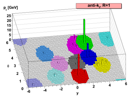
The result of the CMS Particle Flow algorithm is a list of particle candidates that account for all inner-tracker and muon tracks and all above-threshold energy deposits in the calorimeters. These particles are formed into jets using a “clustering algorithm”. The most common algorithm used by CMS is the “anti-kt” algorithm, which is abbreviated “AK”. It iterates over particle pairs and finds the two (i and j) that are the closest in some distance measure and determines whether to combine them:

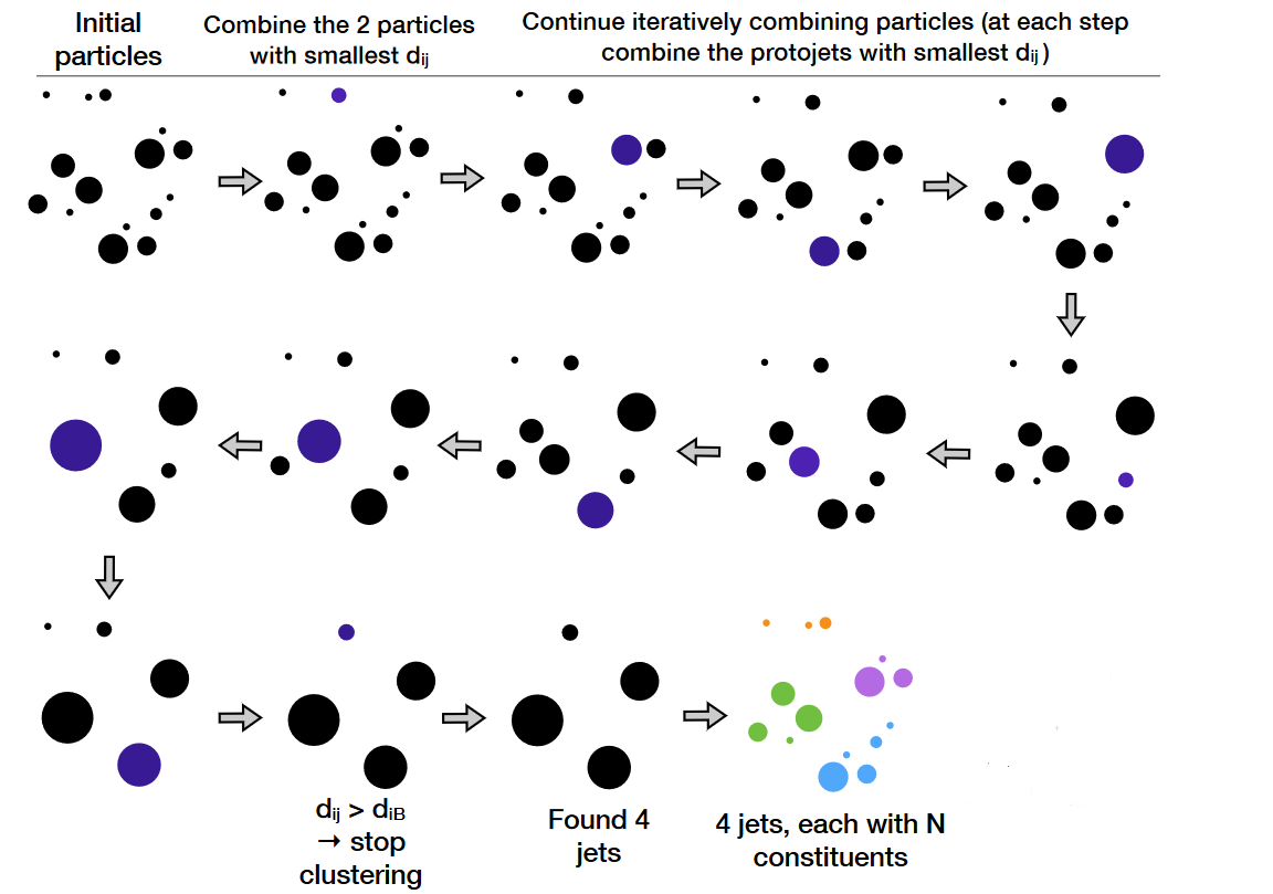
The momentum power (-2) used by the anti-kt algorithm means that higher-momentum particles are clustered first. This leads to jets with a round shape that tend to be centered on the hardest particle. In CMS software this clustering is implemented using the FastJet package.

Pileup
Inevitably, the list of particle flow candidates contains particles that did not originate from the primary interaction point. CMS experiences multiple simultaneous collisions, called “pileup”, during each “bunch crossing” of the LHC, so particles from multiple collisions coexist in the detector. There are various methods to remove their contributions from jets:
- Charged hadron subtraction CHS: all charged hadron candidates are associated with a track. If the track is not associated with the primary vertex, that charged hadron can be removed from the list. CHS is limited to the region of the detector covered by the inner tracker. The pileup contribution to neutral hadrons has to be removed mathematically – more in episode 3!
- PileUp Per Particle Identification (PUPPI, available in Run 2): CHS is applied, and then all remaining particles are weighted based on their likelihood of arising from pileup. This method is more stable and performant in high pileup scenarios such as the upcoming HL-LHC era.
Accessing jets in CMS software
Jets software classes have the same basic 4-vector methods as the objects discussed in the previous lesson. There are two principle ways to interact with jets in the OpenData files: via the reco::Jet class or the pat::Jet class. PAT stands for “Physics Analysis Toolkit”, which is a framework for applying and accessing many common analysis-level algorithms that are used in CMS. The POET features JetAnalyzer.cc to demonstrate working with RECO jets and PatJetAnalyzer.cc to demonstrate working with PAT jets.
In JetAnalyzer.cc
Handle<reco::PFJetCollection> myjets;
iEvent.getByLabel(jetInput, myjets);  // jetInput is "ak5PFJets"

for (reco::PFJetCollection::const_iterator itjet=myjets->begin(); itjet!=myjets->end(); ++itjet){

  ...
  jet_e.push_back(itjet->energy());
  jet_pt.push_back(itjet->pt());
  jet_px.push_back(itjet->px());
  jet_py.push_back(itjet->py());
  jet_pz.push_back(itjet->pz());
  jet_eta.push_back(itjet->eta());
  jet_phi.push_back(itjet->phi());
  jet_ch.push_back(itjet->charge());
  jet_mass.push_back(itjet->mass());

}
In PatJetAnalyzer.cc the jet collection has a different type (and name), and all the energy-related quantities have corrections applied, which will be discussed more in an upcoming lesson.
Handle<std::vector<pat::Jet>> myjets;
iEvent.getByLabel(jetInput, myjets); // jetInput is "selectedPatJetsAK5PFCorr"

for (std::vector<pat::Jet>::const_iterator itjet=myjets->begin(); itjet!=myjets->end(); ++itjet){

  ...
  corr_jet_mass.push_back(itjet->mass());
  corr_jet_e.push_back(itjet->energy());
  corr_jet_px.push_back(itjet->px());
  corr_jet_py.push_back(itjet->py());
  corr_jet_pz.push_back(itjet->pz());
}
Particle-flow jets are not immune to noise in the detector, and jets used in analyses should be filtered to remove noise jets. CMS has defined a Jet ID with criteria for good jets:
The PFlow jets are required to have charged hadron fraction CHF > 0.0 if within tracking fiducial region of |eta| < 2.4, neutral hadron fraction NHF < 1.0, charged electromagnetic (electron) fraction CEF < 1.0, and neutral electromagnetic (photon) fraction NEF < 1.0. These requirements remove fake jets arising from spurious energy depositions in a single sub-detector.
These criteria demonstrate how particle-flow jets combine information across subdetectors. Jets will typically have energy from electrons and photons, but those fractions of the total energy should be less than one. Similarly, jets should have some energy from charged hadrons if they overlap the inner tracker, and all the energy should not come from neutral hadrons. A mixture of energy sources is expected for genuine jets. All of these energy fractions (and more) can be accessed from the jet objects.
MET
Missing transverse momentum is the negative vector sum of the transverse momenta of all particle flow candidates in an event. The magnitude of the missing transverse momentum vector is called missing transverse energy and referred to with the acronym “MET”. Since energy corrections are made to the particle flow jets, those corrections are propagated to MET by adding back the momentum vectors of the original jets and then subtracting the momentum vectors of the corrected jets. This correction is called “Type 1” and is standard for all CMS analyses.
In MetAnalyzer.cc we open the particle flow MET module and extract the magnitude and angle of the MET, the sum of all energy
in the detector, and variables related to the “significance” of the MET. Note that MET quantities have a single value for the
entire event, unlike the objects studied previously.
Handle<reco::PFMETCollection> mymets;
iEvent.getByLabel(metInput, mymets);	// metInput opens "pfMet"

if(mymets.isValid()){
  met_e = mymets->begin()->sumEt();
  met_pt = mymets->begin()->pt();
  met_px = mymets->begin()->px();
  met_py = mymets->begin()->py();
  met_phi = mymets->begin()->phi();

  met_significance = mymets->begin()->significance();
}
If the PAT process has been run, Type 1 corrected MET is also available in MetAnalyzer.cc:
Handle<reco::PFMETCollection> patmets;
iEvent.getByLabel(metInputPat, patmets); // metInputPat opens "pfType1CorrectedMet"

if(patmets.isValid()){
  met_e = patmets->begin()->sumEt();
  met_pt = patmets->begin()->pt();
  met_px = patmets->begin()->px();
  met_py = patmets->begin()->py();
  met_phi = patmets->begin()->phi();
}
MET significance can be a useful tool: it describes the likelihood that the MET arose from noise or mismeasurement in the detector as opposed to a neutrino or similar non-interacting particle. The four-vectors of the other physics objects along with their uncertainties are required to compute the significance of the MET signature. MET that is directed nearly (anti)colinnear with a physics object is likely to arise from mismeasurement and should not have a large significance.
Key Points
Jets are spatially-grouped collections of particles that traversed the CMS detector
Particles from additional proton-proton collisions (pileup) must be removed from jets
Missing transverse energy is the negative vector sum of particle candidates
Many of the class methods discussed for other objects can be used for jets
Triggers
Overview
Teaching: 5 min
Exercises: 0 minQuestions
How are triggers stored using POET?
Objectives
Learn the basics of the POET trigger analyzer
You learned in the pre-exercises about selecting trigger paths and determining pre-scale values. Trigger information can be stored
in POET using the TriggerAnalyzer and TriggObjectAnalyzer.
Trigger Analyzer
The TriggerAnalyzer allows you to store the pass/fail results of certain trigger paths, which can be configured using wildcards. The configuration
also needs to know the names of the trigger collections in the ROOT file.
process.mytriggers = cms.EDAnalyzer('TriggerAnalyzer',
                              processName = cms.string("HLT"),
                              #---- These are example triggers for 2012
                              #---- Wildcards * and ? are accepted (with usual meanings)
                              #---- If left empty, all triggers will run
                              triggerPatterns = cms.vstring("HLT_L2DoubleMu23_NoVertex_v*","HLT_Mu12_v*", "HLT_Photon20_CaloIdVL_v*", "HLT_Ele22_CaloIdL_CaloIsoVL_v*", "HLT_Jet370_NoJetID_v*"),
                              triggerResults = cms.InputTag("TriggerResults","","HLT"),
                              triggerEvent   = cms.InputTag("hltTriggerSummaryAOD","","HLT")
                              )
In TriggerAnalyzer.cc, all available triggers are tested against these patterns for matches, and the matches are stored as a string+integer pairs using std::map<std::string, int>.
For each trigger that matched one of the requested patterns, the name is stored along with a numerical value that gives the “accept bit” (0 or 1) multiplied by the Level-1 and High-Level trigger prescale vales. This is summarized in the tree’s branch title:
  mtree->Branch("triggermap", &trigmap);
  //second  stores the multiplication acceptbit*L1ps*HLTps
  //so, if negative, it means that L1ps couldn't be found.
  //look below in the code to understand the specifics
  mtree->GetBranch("triggermap")->SetTitle("first:name of trigger, second: acceptbit*L1ps*HLTps");
Trigger Object Analyzer
It is also possible to store information about specific physics objects that passed a specific trigger “filter”. Each trigger path will require objects to pass a wide variety of sequential filters in order to arrive at the final pass/fail decision for the event. In analyses it is often interesting to know which physics object actually satisfied the requirement of the trigger. For example, a dilepton search using an electron+muon trigger may wish to reconstruct decays using the specific electron that and specific muon that passed the trigger criteria.
In poet_cfg.py one trigger “filter” can be configured for TriggObjectAnalyzer:
process.mytrigEvent = cms.EDAnalyzer('TriggObjectAnalyzer',
                                     filterName = cms.string("hltL2DoubleMu23NoVertexL2PreFiltered"),
				    )
In TriggObjectAnalyzer.cc, this filter name is used to access a specific list of “keys” and an “object collection” from the trigger summary collection in the ROOT file.
InputTag trigEventTag("hltTriggerSummaryAOD","","HLT"); //make sure have correct process on MC
//data process=HLT, MC depends, Spring11 is REDIGI311X
Handle<trigger::TriggerEvent> mytrigEvent;
iEvent.getByLabel(trigEventTag,mytrigEvent);

numtrigobj = 0;
trigobj_e.clear();
trigobj_pt.clear();
trigobj_px.clear();
trigobj_py.clear();
trigobj_pz.clear();
trigobj_eta.clear();
trigobj_phi.clear();

trigger::size_type filterIndex = mytrigEvent->filterIndex(edm::InputTag(filterName_,"",trigEventTag.process()));
if(filterIndex<mytrigEvent->sizeFilters()){
  const trigger::Keys& trigKeys = mytrigEvent->filterKeys(filterIndex);
  const trigger::TriggerObjectCollection & trigObjColl(mytrigEvent->getObjects());
We can then loop through the list of keys and access the object with that key from the object collection. Storing this object’s basic 4-vector properties allows the analyst to find the electron, muon, tau, jet, etc that is closest to the trigger object in angular separation.
  //now loop of the trigger objects passing filter
  for(trigger::Keys::const_iterator keyIt=trigKeys.begin();keyIt!=trigKeys.end();++keyIt){
    const trigger::TriggerObject trigobj = trigObjColl[*keyIt];

    //do what you want with the trigger objects, you have
    //eta,phi,pt,mass,p,px,py,pz,et,energy accessors
    trigobj_e.push_back(trigobj.energy());
    trigobj_pt.push_back(trigobj.pt());
    trigobj_px.push_back(trigobj.px());
    trigobj_py.push_back(trigobj.py());
    trigobj_pz.push_back(trigobj.pz());
    trigobj_eta.push_back(trigobj.eta());
    trigobj_phi.push_back(trigobj.phi());

    numtrigobj=numtrigobj+1;
  }
}//end filter size check
For jets, a trigger object matched within the size of the jet cone (perhaps dR < 0.5) would constitute a match. For leptons and photons a smaller separation is typically used, perhaps dR < 0.2. The exact requirements will be analysis specific!
Key Points
Trigger paths are stored as a map with names paired to prescale values
4-vector information is stored for objects matching a specific, configurable, trigger filter
15 minute break
Overview
Teaching: 0 min
Exercises: 15 minQuestions
Which type of coffee will you drink on your break?
Objectives
Acquire coffee. Drink coffee.
Take a break!
Key Points
Any type of coffee is refreshing after so much concentrated learning.
Basic objects hands-on
Overview
Teaching: 0 min
Exercises: 40 minQuestions
How can I navigate the physics object references to compute identification criteria?
How can I separate events with and without invisible particles?
Objectives
Practice expanding identification criteria beyond POET defaults.
Practice interacting with ROOT file output from POET.
Choose your exercise! The first several exercises all relate to manipulating identification criteria for muons, taus, or jets. Please complete one of them.
Exercise 1 option A: add alternate muon IDs and isolation corrections
Using the documentation on the TWiki page:
- adjust the 0.4-cone muon isolation calculation to apply the “DeltaBeta” pileup correction.
- add the pass/fail information about the Loose identification working point.
- try to recreate the Tight identification working point from detector information criteria!
Solution:
The DeltaBeta correction for pileup involves subtracting off half of the pileup contribution that can be accessed from the “iso04” object already being used:
if (itmuon->isPFMuon() && itmuon->isPFIsolationValid()) {
 auto iso04 = itmuon->pfIsolationR04();
 muon_pfreliso04all.push_back((iso04.sumChargedHadronPt + iso04.sumNeutralHadronEt + iso04.sumPhotonEt - 0.5*iso04.sumPUPt)/itmuon->pt());
To add new variables we need to check four code locations: declarations, branches, vector clearing, and vector filling. You might add Loose ID beneath the existing Tight and Soft IDs in each section:
std::vector<float> muon_softid; std::vector<float> muon_looseid;mtree->Branch("muon_softid",&muon_softid); mtree->GetBranch("muon_softid")->SetTitle("soft cut-based ID"); mtree->Branch("muon_looseid",&muon_looseid); mtree->GetBranch("muon_looseid")->SetTitle("loose cut-based ID");muon_softid.clear(); muon_looseid.clear();muon_softid.push_back(muon::isSoftMuon(*itmuon, *vertices->begin())); muon_looseid.push_back(muon::isLooseMuon(*itmuon));The TWiki also gives the member functions needed to reconstruct the muon ID. We can see from the built-in tightID method that a vertex is needed for some of the criteria:
muon::isTightMuon(*it, *vertices->begin()). To learn more about the vertex collection you can refer toVertexAnalyzer.cc.std::vector<bool> muon_isTightByHand; if( it->isGlobalMuon() && it->isPFMuon() && it->globalTrack()->normalizedChi2() < 10. && it->globalTrack()->hitPattern().numberOfValidMuonHits() > 0 && it->numberOfMatchedStations() > 1 && fabs(it->muonBestTrack()->dxy(vertices->begin()->position())) < 0.2 && fabs(it->muonBestTrack()->dz(vertex->position())) < 0.5 && it->innerTrack()->hitPattern().numberOfValidPixelHits() > 0 && it->innerTrack()->hitPattern().trackerLayersWithMeasurement() > 5) { muon_isTightByHand.push_back(true); }
Exercise 1 option B: add alternate tau IDs
Many other tau discriminants exist. Based on information from the TWiki, save the values for some discriminants that are based on multivariate analysis techniques.
Solution:
The TWiki describes Loose/Medium/Tight ID levels for a “IsolationMVA” and “IsolationMVA2” algorithms. They can be accessed like the other tau IDs, but you might need to refer to the output of
edmDumpEventContentto find the exact form of the InputTag name.Add declarations:
std::vector<bool> tau_idisoMVA2loose;
std::vector<bool> tau_idisoMVA2tight;
Add branches:
mtree->Branch("tau_idisoMVA2loose",&tau_idisoMVA2loose);
mtree->GetBranch("tau_idisoMVA2loose")->SetTitle("tau id loose isolation from MVA2");
// ...etc for other ID...
Create handles and get the information from the input file:
Handle<PFTauCollection> taus;
iEvent.getByLabel(InputTag("hpsPFTauProducer"), taus);

Handle<PFTauDiscriminator> tausLooseIso, tausVLooseIso, tausMediumIso, tausTightIso,
                          tausDecayMode, tausRawIso, tausTightEleRej,
			     tausTightMuonRej, tausLooseIsoMVA2, tausTightIsoMVA2;

// new things only
iEvent.getByLabel(InputTag("hpsPFTauDiscriminationByLooseIsolationMVA2"),tausLooseIsoMVA2);
iEvent.getByLabel(InputTag("hpsPFTauDiscriminationByTightIsolationMVA2"),tausTightIsoMVA2);
Clear the vectors at the beginning of each event:
tau_idisoMVA2loose.clear()
tau_idisoMVA2tight.clear()
And finally, access the discriminator from the second element of the pair:
tau_idisoMVA2loose.push_back(tausLooseIsoMVA2->operator[](idx).second);
tau_idisoMVA2tight.push_back(tausTightIsoMVA2->operator[](idx).second);
Exercise 1 option C: apply noise jet ID
Use the cms-sw github repository to learn the methods available for pat::Jets (hint: the header file is included from
PatJetAnalyzer.cc). Implement the jet ID and reject jets that do not pass. Rejection means that information about these jets will not be stored in any of the tree branches.Solution
The header file we need is for particle-flow jets:
interface/Jet.hfrom the link given. It shows many functions like this:/// chargedHadronEnergyFraction (relative to uncorrected jet energy) float chargedHadronEnergyFraction() const {return chargedHadronEnergy()/((jecSetsAvailable() ? jecFactor(0) : 1.)*energy());}These functions give the energy from a certain type of particle flow candidate as a fraction of the jet’s total energy. We can apply the conditions given to reject jets from noise at the same time we apply a momentum threshold:
for (std::vector<pat::Jet>::const_iterator itjet=myjets->begin(); itjet!=myjets->end(); ++itjet){
 if (itjet->chargedHadronEnergyFraction() > 0 && itjet->neutralHadronEnergyFraction() < 1.0 &&
     itjet->electronEnergyFraction() < 1.0 && itjet->photonEnergyFraction() < 1.0){

   // calculate things on jets
 }
}
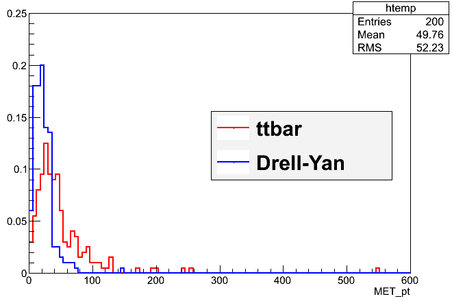
Exercise 2: real and fake MET
Compile all your changes to POET so far and run 400 events from two different simulation samples. One test file contains top quark pair events, so some events will have leptonic decays that include neutrinos and some events will not. The other test file contains Drell-Yan events without neutrinos. Review TTree::Draw from the pre-exercises – can you draw histograms of MET versus MET significance and infer which events have leptonic decays?
$ scram b
$ # edit python/poet_cfg.py to run over 400 events from the ttbar simulation test file.
$ cmsRun python/poet_cfg.py
$ # edit python/poet_cfg.py to use this input file: root://eospublic.cern.ch//eos/opendata/cms/MonteCarlo2012/Summer12_DR53X/DYJetsToLL_M-50_TuneZ2Star_8TeV-madgraph-tarball/AODSIM/PU_RD1_START53_V7N-v1/20000/003063B7-4CCF-E211-9FED-003048D46124.root, and to save a file called myoutput_DY.root
$ cmsRun python/poet_cfg.py
$ root -l myoutput.root
[0] TTree *ttbar = (TTree*)_file0->Get("mymets/Events");
[1] TFile *_file1 = TFile::Open("myoutput_DY.root");
[2] TTree *dy = (TTree*)_file1->Get("mymets/Events");
[3] ttbar->Draw("...a branch name...", "...any cuts go here...", "norm")
[4] dy->Draw("...a branch name...", "...any cuts go here...", "norm pe same")
Solution
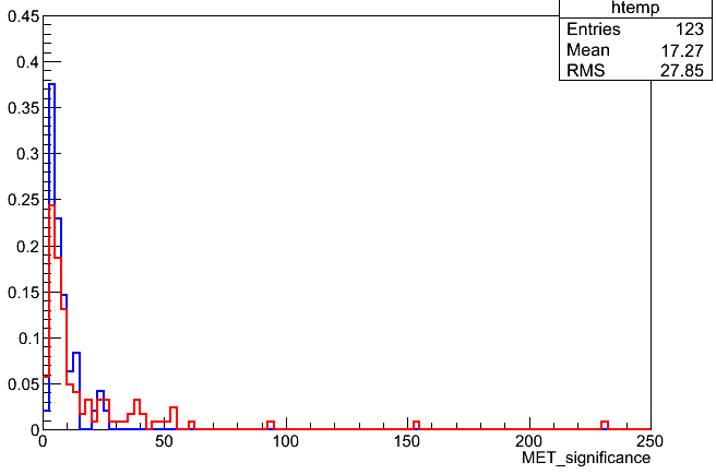
The difference between the Drell-Yan events with primarily fake MET and the top pair events with primarily genuine MET can be seen by drawing
MET_ptor by drawingMET_significance. In both distributions the Drell-Yan events have smaller values than the top pair events.
Key Points
All physics objects have multiple identification and isolation schemes.
POET implements the most common identification and isolation criteria used in analyses.
MET exists in all events, but significant differences can be seen between samples with and without real MET.
Come back tomorrow morning!
Overview
Teaching: 0 min
Exercises: 0 minQuestions
Objectives
The Challenge session for this lesson is schedule for Tuesday at 15:10 CERN time. See you then!
Key Points
Basic objects challenge
Overview
Teaching: 0 min
Exercises: 45 minQuestions
How should I construct selection criteria for a physics analysis?
Objectives
Combine trigger, identification, and isolation information into a full selection for a specific physics process.
All of the trigger and physics object information from this lesson is combined when designing the event selection procedure for a physics analysis.
Workshop analysis example: H -> tau tau
Later in the workshopw we will use a search for Higgs bosons as an example analysis. The signal for this search is one Higgs boson that decays to two tau leptons, with one tau lepton decaying hadronically and the other tau lepton decaying to a muon and neutrinos.
Your analysis example
What is a physics process that you might study? Let’s design a possible CMS event selection. If your process includes a particle with multiple possible decay modes, choose one (or a small group of very similar decay modes) as a test case for this challenge.
For the Higgs search and/or your own process of interest, use the information you have gained about triggers and physics objects to sketch out a possible event selection for your analysis.
Signal
Which final state particles would you expect to observe in the detector from your “signal” process?
Based on these particles, consider:
- Which trigger or triggers would be useful to make sure your signal events are represented in the dataset?
- Which objects should you require in each event?
- What kinematic criteria might you requier for each object? (momentum, angular regions, etc)
- What quality criteria might you require for each object? (identification, isolation)
- Are there any correlations between your objects that you might exploit?
Background
Which SM backgrounds could easily mimic your signal, given a few extra physics objects, or a few missing physics objects?
Based on these processes, consider:
- Which background simulations should you include in your study?
- Should you apply any upper or lower limits on the numbers of certain physics objects in your events?
- Are there any objects you should veto from your events?
- What quality criteria might you choose for vetoing objects?
Solutions
In the final session for this lesson we will go over the actual analysis choices for H -> tau tau and discuss approaches for some physics processes you chose for this challenge.
Key Points
Come back for the solutions session tomorrow!
15 minute break
Overview
Teaching: 0 min
Exercises: 15 minQuestions
Which type of coffee will you drink on your break?
Objectives
Acquire coffee. Drink coffee.
Take a break!
Key Points
Any type of coffee is refreshing after so much concentrated learning.
Solutions and questions
Overview
Teaching: 40 min
Exercises: minQuestions
How should I construct selection criteria for a physics analysis?
Objectives
Combine trigger, identification, and isolation information into a full selection for a specific physics process.
All of the trigger and physics object information from this lesson is combined when designing the event selection procedure for a physics analysis.
Workshop analysis example: H -> tau tau
Later in the workshopw we will use a search for Higgs bosons as an example analysis. The signal for this search is one Higgs boson that decays to two tau leptons, with one tau lepton decaying hadronically and the other tau lepton decaying to a muon and neutrinos.
Your analysis example
What is a physics process that you might study? Let’s design a possible CMS event selection. If your process includes a particle with multiple possible decay modes, choose one (or a small group of very similar decay modes) as a test case for this challenge.
For the Higgs search and/or your own process of interest, use the information you have gained about triggers and physics objects to sketch out a possible event selection for your analysis.
Signal
Which final state particles would you expect to observe in the detector from your “signal” process?
Solution
For the Higgs -> tau tau search we expect one hadronic tau object, one muon, and MET from the Higgs boson decay, and potentially two or more jets if the Higgs boson was produced via vector boson fusion.


Based on these particles, consider:
- Which trigger or triggers would be useful to make sure your signal events are represented in the dataset?
Solution
This analysis is perfect for a “cross trigger” that selects more than one object! The trigger used in this example is
HLT_IsoMu17_eta2p1_LooseIsoPFTau20, requiring both a muon and a tau.
- Which objects should you require in each event?
Solution
Certainly at least 1 muon and 1 hadronic tau! An analyst targeting VBF production might also require at least 2 jets, especially jets that were detected near the endcaps of the detector. A MET requirement is more tricky to choose: since the neutrinos involved in this event likely do not carry away very large momenta, imposing a MET threshold may not significantly improve the selection.
- What kinematic criteria might you requier for each object? (momentum, angular regions, etc)
Solution
The trigger criterion imposes some constraints: we will lose muons with pT below 17 GeV or large pseudorapidity, and hadronic taus with pT below 20 GeV. Since there is typically some “turn-on” in the efficiency of the trigger selection, it would be safer to add a momentum buffer to our selection. This analysis requires:
- 1 or more muons with pT > 20 GeV and absolute eta < 2.1
- 1 or more hadronic taus with pT > 30 GeV and absolute eta < 2.4
- What quality criteria might you require for each object? (identification, isolation)
Solution
Tau selection:
- We learned from the tau reference twiki that we should always require
taus_iddecaymodeto be true.- The trigger adds an extra criterion: we should at least require that the
taus_idisolooseflag is true. In fact, the version of this analysis on the OpenData portal requires that even thetaus_idisotightflag is true.- We want to protect against selecting taus that were actually misidentified electrons or muons. This is done by requiring
taus_idantieletightandtaus_idantimutightto be true.Muon selection:
- The ID is not restricted by the trigger, but the “tight” working point is by far the most popular choice for any signal muons.
- Since the muon is not expected to be produced very near to a jet or the tau, this analysis requires that the
muon_pfreliso04allisolation be < 0.1.
- Are there any correlations between your objects that you might exploit?
Solution
Since the Higgs boson is neutral, we expect that the muon and tau lepton have opposite charges. This requirement can help reduce background events with unassociated muon and tau objects.
Background
Which SM backgrounds could easily mimic your signal, given a few extra physics objects, or a few missing physics objects?
Solution
The backgrounds for the Higgs search are described on the OpenData Portal page
Based on these processes, consider:
- Which background simulations should you include in your study?
Solution
The most important sample to include is Z -> tau tau, since the final state is effectively identical to the Higgs boson case. Other Z boson, W boson, and top quark samples will be included. Multijet (“QCD”) background simulation is often not used in final results because of the difficulty in modeling pure QCD interactions, so this background is more often estimated using data in alternate selection regions (“control regions”).
- Should you apply any upper or lower limits on the numbers of certain physics objects in your events?
Solution
It is often useful to select events with exactly a certain number of objects rather than at least a certain number. Close study of background versus signal processes in simulation can help show which choices are best for a certain signal. In this case, since muons and tau combinations are rare from proton collisions, we will simply select the best single muon and tau to reconstruct as a Higgs boson rather than imposing limits.
- Are there any objects you should veto from your events? What quality criteria might you choose?
Solution
In a sample list consisting of Higgs or Z -> tau tau, Z -> leptons, W -> leptons, and top pairs -> (bW)(bW) -> bb+leptons, one object stands out: b-tagged jets. The top pair background in this analysis can be dramatically reduced by rejecting events with any b-tagged jets. Typically a loose requirement is used on veto objects so that efficiency for rejecting background-heavy events is highest, but this is a case-by-case decision.
In the published analysis, event categories targeting VBF Higgs production vetoed additional jets in the central region of the detector since those are inconsistent with a VBF hypothesis. Events are also categorized based on which leptons (muons or electrons) appear in the event – if not using multiple categories, a muon analysis might veto on the presence of electrons to reduce backgrounds.
- Are there any correlations between objects in background that might be useful for rejection?
Solution
Looking back to the background list, the W boson background has the unique feature that a single neutrino is expected from its decay products. The transverse mass (see equation 2) constructed from the muon and MET is typically near the W boson mass for this background, while it should have small values in signal since the muon and the tau-decay neutrinos are not associated. This analysis requires the muon+MET transverse mass to be < 30 GeV to reject W boson background.
Key Points
Triggers usually impose various kinematic restrictions on objects of interest.
Final state objects produced promptly from the proton collision are typically required to have significant momentum, tight ID quality, and to be isolated (depending on the topology of the physics process.
Veto objects are typically selected using looser criteria so that the efficiency of the veto is very high.
Correlations between objects can be used either to select specifically for signal events or reject background events.