
All in One View
Content from Intro to CMS Physics Objects
Last updated on 2026-07-16 | Edit this page
Estimated time: 5 minutes
Overview
Questions
- What do we call physics objects in CMS?
- How are physics objects reconstructed?
- How are physics objects represented in NanoAOD?
Objectives
- Learn about the different physics objects in CMS and get briefed on their reconstruction
- Learn more about the collection structure of NanoAOD
Overview
The CMS experment is a giant detector that acts like a camera that “photographs” particle collisions, allowing us to interpret their nature.
Certainly, we cannot directly observe all the particles created in the collisions because some of them decay very quickly or simply do not interact with our detector. However, we can infer their presence. If they decay to more stable particles and interact with the material of the detector, they leave signals that CMS can record. These signals are used to determine the presence of specific types of particles moving through the detector – we call these, physics objects.
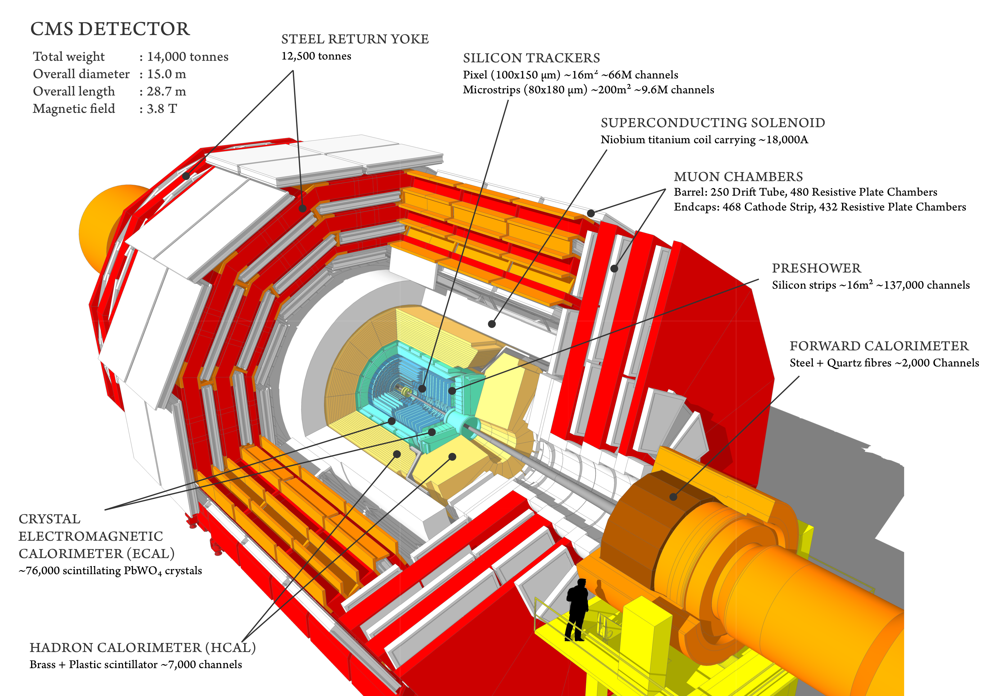
The CMS detector has many many sensors of different kinds that can detect signals from particles passing through. Take a look at the CMS experiment in the image below. This is a good recent video that you can watch later to get a quick feeling of how CMS looks now in Run 3.
Physics objects can be:
- electrons
- muons
- photons
- “jets” (cones of energy from particles made of quarks)
- tau leptons
- missing transverse momentum
On the CERN Open Portal (CODP) site you can find a more detailed description of these physics objects and a list of them corresponding to 2010, 2011/2012, and 2015/2016 releases of open data.
In this workshop we will focus on working with open data from the latest 2016 release from Run 2. This release included the NanoAOD file format that contains the most commonly used physics object information in a standard ROOT tree.
Physics Objects reconstruction
Physics objects are mainly reconstructed using methods like clustering adjacent signals and linking information between different CMS detector components. For instance, electromagnetic objects (electrons or photons) are reconstructed by linking tracks from the inner tracking detectors with energy clusters in the electromagnetic calorimeter.
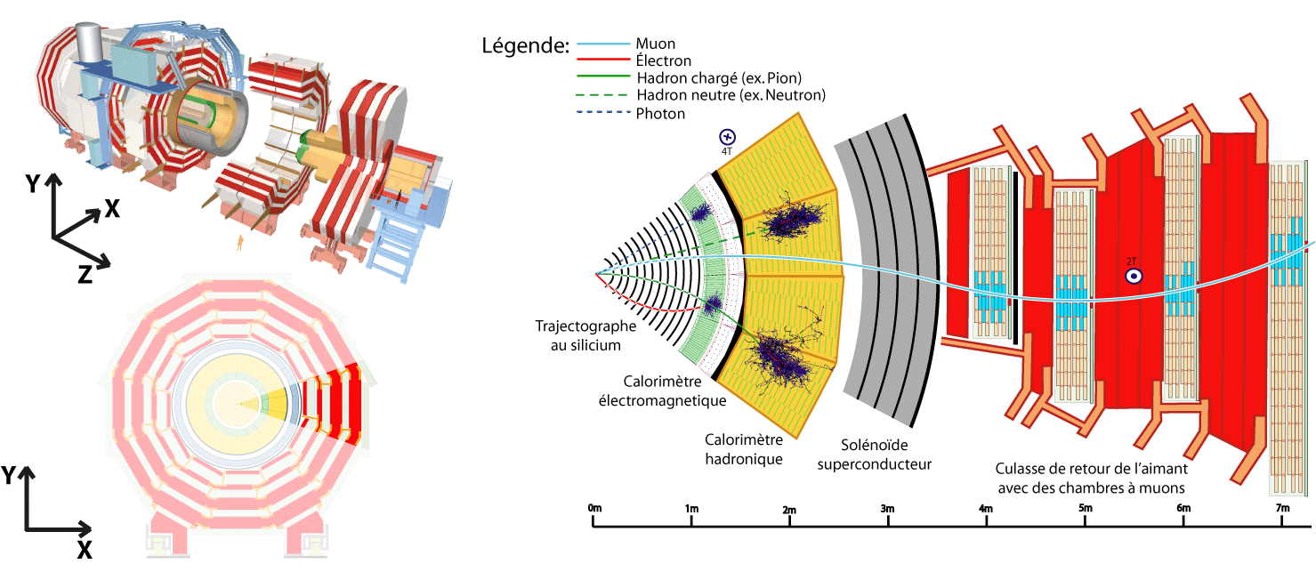
These actions are essential parts of the so-called Particle Flow (PF) algorithm.
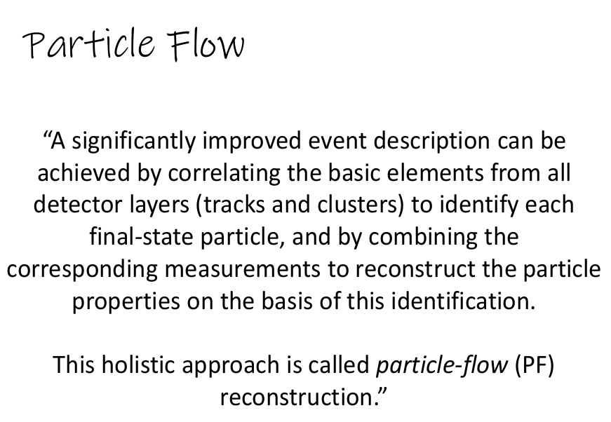
The particle-flow (PF) algorithm aims at reconstructing and identifying all stable particles in the event, i.e., electrons, muons, photons, charged hadrons and neutral hadrons, with a thorough combination of all CMS sub-detectors in order to best determine their direction, energy and particle type. This list of individual particles is then used to build jets, to determine the missing transverse energy (which gives an estimate of the direction and energy of the neutrinos and other invisible particles), to reconstruct and identify tau leptons from their decay products, and more.
The PF algorithm is written in C++ and is part of the CMSSW software that is required to analyze any open data in the earlier AOD or MiniAOD formats. For more information about the PF algorithm you can visit a lesson from an earlier workshop: Advanced Tools lesson. The CMS open data from 2016 contains some data samples in the NanoAOD format that have been supplemented with particle flow information: nanoad-pf samples.
- Physics objects are the final abstraction in the detector that can be associated to physical entities like particles.
- NanoAOD stores physics object properties as branches of a ROOT tree, linked by common name prefixes.
Content from Electrons & Photons
Last updated on 2026-07-16 | Edit this page
Estimated time: 10 minutes
Overview
Questions
- What are electromagnetic objects
- How are electrons treated in CMS?
- What variables are available in NanoAOD?
Objectives
- Understand what electromagnetic objects are in CMS
- Learn electron member functions for common track-based quantities
- Learn variables for identification and isolation of electrons
- Learn variables for electron detector-related quantities
Motivation
In this workshop we will do some simple analysis examples using NanoAOD Open Data. Physics objects that are detected in CMS have their properties measured and stored in the CMS data files. This and the following pages will introduce the different physics objects more deeply and try to explain several of the most important “branches” in NanoAOD ROOT “trees” for each type of object.
Electromagnetic objects
We call photons and electrons electromagnetic particles because they leave most of their energy in the electromagnetic calorimeter (ECAL) so they share many common properties.
Many of the different hypothetical exotic particles for which CMS scientists are searching are unstable. Some of these particles can transform, or decay, into electrons, photons, or both. Electrons and photons are also standard tools to measure better and understand the properties of already known particles. For example, one way to find a Higgs Boson is by looking for signs of either two photons or four electrons in the debris of high energy collisions. Because electrons and photons are crucial in so many different scenarios, the physicists in the CMS collaboration make sure to do their best to reconstruct and identify these objects.
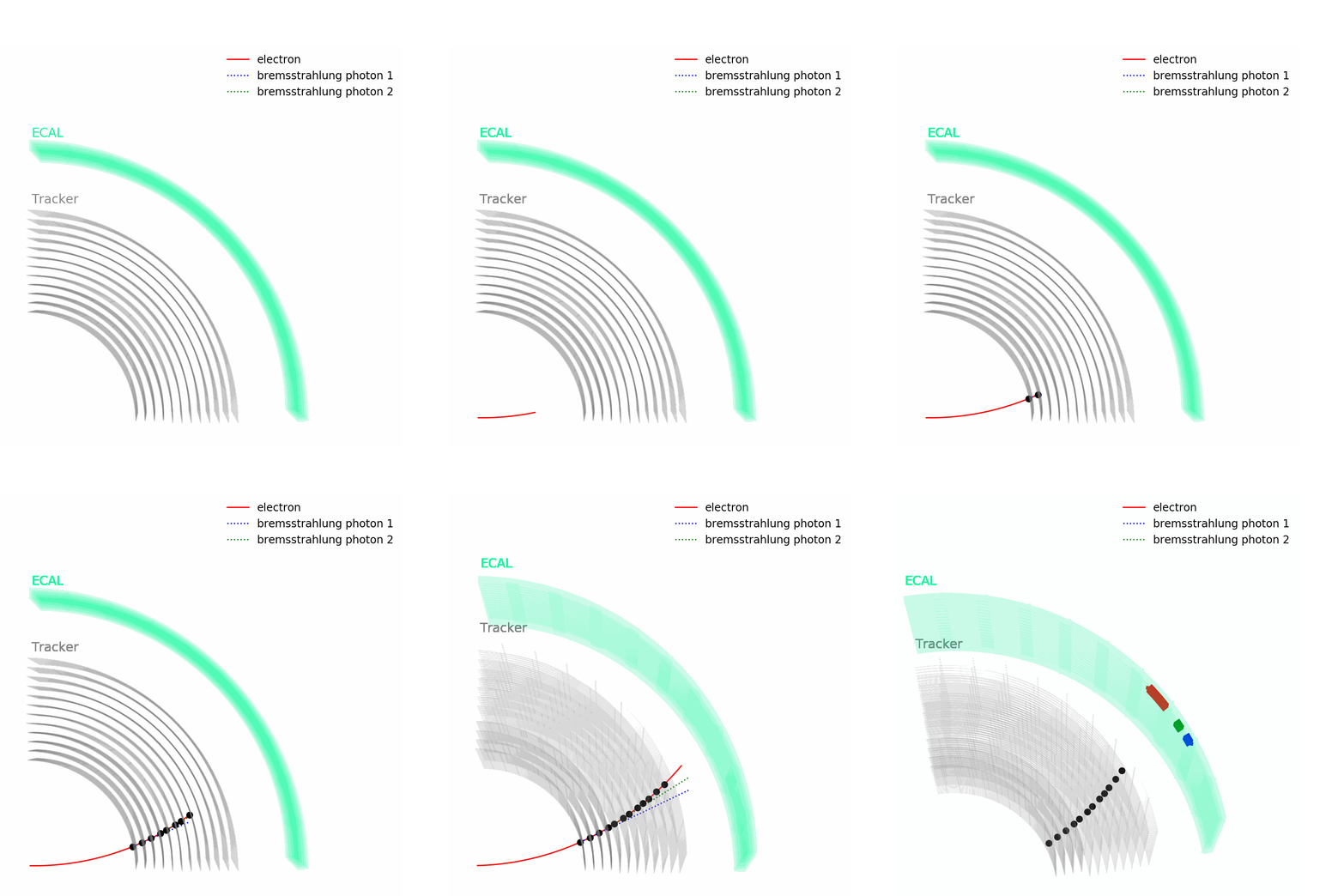
As depicted in the figure above, tracks – from the pixel and silicon tracker systems – as well as ECAL energy deposits are used to identify the passage of electrons in CMS. Being charged, the solid red electron trajectory curves inside the CMS magnetic field. Photons (depicted with dashed lines above) are similar objects but with no tracks. Sophisticated algorithms are run in the reconstruction to take into account subtleties related to the identification of an electromagnetic particle. An example is the convoluted showering of sub-photons and sub-electrons that can reach the ECAL due to bremsstrahlung and photon conversions – in the animation, all three energy deposits shown in the ECAL would be grouped together as coming from one electron object.
From the tracks and energy clusters we can measure the electromagnetic particle’s momentum and energy as well as other properties that help analysts understand better their quality and origin.
Electron variables in NanoAOD
One example of a NanoAOD dataset on the Open Data Portal is the SingleElectron dataset.
The “Dataset Semantics” section has a link to the variable
list webpage. Each “collection” of objects in the NanoAOD file is
linked by a common naming scheme (ex: Electron_*). The
individual variables are shown in a table that includes the branch name,
the data type, and a brief descriptive comment.
| Object property | Type | Description |
|---|---|---|
| Electron_charge | Int_t | electric charge |
| Electron_cleanmask | UChar_t | simple cleaning mask with priority to leptons |
| Electron_convVeto | Bool_t | pass conversion veto |
| Electron_cutBased | Int_t | cut-based ID Fall17 V2 (0:fail, 1:veto, 2:loose, 3:medium, 4:tight) |
| Electron_cutBased_HEEP | Bool_t | cut-based HEEP ID |
| Electron_dEscaleDown | Float_t | ecal energy scale shifted 1 sigma down (adding gain/stat/syst in quadrature) |
| Electron_dEscaleUp | Float_t | ecal energy scale shifted 1 sigma up(adding gain/stat/syst in quadrature) |
| Electron_dEsigmaDown | Float_t | ecal energy smearing value shifted 1 sigma up |
| Electron_dEsigmaUp | Float_t | ecal energy smearing value shifted 1 sigma up |
| Electron_deltaEtaSC | Float_t | delta eta (SC,ele) with sign |
| Electron_dr03EcalRecHitSumEt | Float_t | Non-PF Ecal isolation within a delta R cone of 0.3 with electron pt > 35 GeV |
| Electron_dr03HcalDepth1TowerSumEt | Float_t | Non-PF Hcal isolation within a delta R cone of 0.3 with electron pt > 35 GeV |
| Electron_dr03TkSumPt | Float_t | Non-PF track isolation within a delta R cone of 0.3 with electron pt > 35 GeV |
| Electron_dr03TkSumPtHEEP | Float_t | Non-PF track isolation within a delta R cone of 0.3 with electron pt > 35 GeV used in HEEP ID |
| Electron_dxy | Float_t | dxy (with sign) wrt first PV, in cm |
| Electron_dxyErr | Float_t | dxy uncertainty, in cm |
| Electron_dz | Float_t | dz (with sign) wrt first PV, in cm |
| Electron_dzErr | Float_t | dz uncertainty, in cm |
| Electron_eCorr | Float_t | ratio of the calibrated energy/miniaod energy |
| Electron_eInvMinusPInv | Float_t | 1/E_SC - 1/p_trk |
| Electron_energyErr | Float_t | energy error of the cluster-track combination |
| Electron_eta | Float_t | eta |
| Electron_hoe | Float_t | H over E |
| Electron_ip3d | Float_t | 3D impact parameter wrt first PV, in cm |
| Electron_isPFcand | Bool_t | electron is PF candidate |
| Electron_jetIdx | Int_t | (index to Jet) index of the associated jet (-1 if none) |
| Electron_jetNDauCharged | UChar_t | number of charged daughters of the closest jet |
| Electron_jetPtRelv2 | Float_t | Relative momentum of the lepton with respect to the closest jet after subtracting the lepton |
| Electron_jetRelIso | Float_t | Relative isolation in matched jet (1/ptRatio-1, pfRelIso04_all if no matched jet) |
| Electron_lostHits | UChar_t | number of missing inner hits |
| Electron_mass | Float_t | mass |
| Electron_miniPFRelIso_all | Float_t | mini PF relative isolation, total (with scaled rho*EA PU corrections) |
| Electron_miniPFRelIso_chg | Float_t | mini PF relative isolation, charged component |
| Electron_mvaFall17V2Iso | Float_t | MVA Iso ID V2 score |
| Electron_mvaFall17V2Iso_WP80 | Bool_t | MVA Iso ID V2 WP80 |
| Electron_mvaFall17V2Iso_WP90 | Bool_t | MVA Iso ID V2 WP90 |
| Electron_mvaFall17V2Iso_WPL | Bool_t | MVA Iso ID V2 loose WP |
| Electron_mvaFall17V2noIso | Float_t | MVA noIso ID V2 score |
| Electron_mvaFall17V2noIso_WP80 | Bool_t | MVA noIso ID V2 WP80 |
| Electron_mvaFall17V2noIso_WP90 | Bool_t | MVA noIso ID V2 WP90 |
| Electron_mvaFall17V2noIso_WPL | Bool_t | MVA noIso ID V2 loose WP |
| Electron_mvaTTH | Float_t | TTH MVA lepton ID score |
| Electron_pdgId | Int_t | PDG code assigned by the event reconstruction (not by MC truth) |
| Electron_pfRelIso03_all | Float_t | PF relative isolation dR=0.3, total (with rho*EA PU corrections) |
| Electron_pfRelIso03_chg | Float_t | PF relative isolation dR=0.3, charged component |
| Electron_phi | Float_t | phi |
| Electron_photonIdx | Int_t | (index to Photon) index of the associated photon (-1 if none) |
| Electron_pt | Float_t | p_{T} |
| Electron_r9 | Float_t | R9 of the supercluster, calculated with full 5x5 region |
| Electron_scEtOverPt | Float_t | (supercluster transverse energy)/pt-1 |
| Electron_seedGain | UChar_t | Gain of the seed crystal |
| Electron_sieie | Float_t | sigma_IetaIeta of the supercluster, calculated with full 5x5 region |
| Electron_sip3d | Float_t | 3D impact parameter significance wrt first PV, in cm |
| Electron_tightCharge | Int_t | Tight charge criteria (0:none, 1:isGsfScPixChargeConsistent, 2:isGsfCtfScPixChargeConsistent) |
| Electron_vidNestedWPBitmap | Int_t | VID compressed bitmap (MinPtCut,GsfEleSCEtaMultiRangeCut,GsfEleDEtaInSeedCut,GsfEleDPhiInCut,GsfEleFull5x5SigmaIEtaIEtaCut,GsfEleHadronicOverEMEnergyScaledCut,GsfEleEInverseMinusPInverseCut,GsfEleRelPFIsoScaledCut,GsfEleConversionVetoCut,GsfEleMissingHitsCut), 3 bits per cut |
| Electron_vidNestedWPBitmapHEEP | Int_t | VID compressed bitmap (MinPtCut,GsfEleSCEtaMultiRangeCut,GsfEleDEtaInSeedCut,GsfEleDPhiInCut,GsfEleFull5x5SigmaIEtaIEtaWithSatCut,GsfEleFull5x5E2x5OverE5x5WithSatCut,GsfEleHadronicOverEMLinearCut,GsfEleTrkPtIsoCut,GsfEleEmHadD1IsoRhoCut,GsfEleDxyCut,GsfEleMissingHitsCut,GsfEleEcalDrivenCut), 1 bits per cut |
| nElectron | UInt_t | slimmedElectrons after basic selection (pt > 5 ) |
Electron 4-vector and track information
All CMS physics objects contain basic 4-vector information: transverse momentum, pseudorapidity (related to angle from one proton beam to the other), azimuthal angle (angle around the cylinder of CMS), and mass or energy. This information can easily be converted into a 4-vector of px, py, pz, and energy.
| Object property | Type | Description |
|---|---|---|
| Electron_eta | Float_t | eta |
| Electron_mass | Float_t | mass |
| Electron_phi | Float_t | phi |
| Electron_pt | Float_t | p_T, transverse momentum |
Most charged physics objects are also connected to tracks from the
CMS tracking detectors, and therefore the electric charge can be
identified from the track curvature. Electron charge can be computed
from 3 unique algorithms, so a tightCharge variable exists
to show when multiple of the charge determinations agree. Information
from tracks provides other kinematic quantities that are common to
multiple types of objects. It is often interesting to check the
impact parameter of a charged object’s track with
respect to the primary collision vertex, since this gives a good idea of
whether or not that particle emerged directly from that particular
collision or not. We can access the impact parameters in the xy-plane
(dxy or d0) and along the beam axis
(dz), as well as their respective uncertainties. There is
also a 3D impact parameter significance that is very useful for
identifying leptons that emerged from a heavy flavor hadron decay, since
those leptons will usually have a larger 3D impact parameter.
| Object property | Type | Description |
|---|---|---|
| Electron_charge | Int_t | electric charge |
| Electron_dxy | Float_t | dxy (with sign) wrt first PV, in cm |
| Electron_dxyErr | Float_t | dxy uncertainty, in cm |
| Electron_dz | Float_t | dz (with sign) wrt first PV, in cm |
| Electron_dzErr | Float_t | dz uncertainty, in cm |
| Electron_sip3d | Float_t | 3D impact parameter significance wrt first PV, in cm |
| Electron_tightCharge | Int_t | Tight charge criteria (0:none, 1:isGsfScPixChargeConsistent, 2:isGsfCtfScPixChargeConsistent) |
Track-based info for photons
Note: in the case of Photons, since they are neutral objects, they do
not have a direct track link. While the charge variable
exists for all objects, it is not used in photon analyses.
Detector information for identification
The most signicant difference between a list of certain particles from a simulation and a list of the corresponding physics objects from CMS data is likely the inherent uncertainty in the reconstruction. Selection of “a muon” or “an electron” for analysis requires algorithms designed to separate “real” objects from “fakes”. These are called identification algorithms.
Other algorithms are designed to measure the amount of energy deposited near the object, to determine if it was likely produced near the primary interaction (typically little nearby energy), or from the decay of a longer-lived particle (typically a lot of nearby energy). These are called isolation algorithms. Many types of isolation algorithms exist to deal with unique physics cases!
Both types of algorithms function using working points that are described on a spectrum from “loose” to “tight”. Working points that are “looser” tend to have a high efficiency for accepting real objects, but perhaps a poor rejection rate for “fake” objects. Working points that are “tighter” tend to have lower efficiencies for accepting real objects, but much better rejection rates for “fake” objects. The choice of working point is highly analysis dependent! Some analyses value efficiency over background rejection, and some analyses are the opposite.
The standard identification and isolation algorithm results can be accessed from the physics object classes.
Multivariate Electron Identification (MVA)
In the Multi-variate Analysis (MVA) approach, simple machine learning networks are trained on multiple parameters of the electron object, and the network’s output value (which typically spans from 0 to 1) can be used to separate real electrons from fake electrons. Analysts choose a particular numerical value to use as the division point between real objects (with values higher that the cut) and fake objects (with values lower than the cut). There are two basic types of MVAs that are were trained by CMS for 2016 electrons:
- MVA with isolation: the MVA includes standard particle-flow isolation as one of the variables used for training. This MVA is well suited for analyses considering typical prompt electrons that are likely to be isolated from jets or other objects.
- MVA without isolation: no isolation variables are included for training. This MVA is better suited for analyses in which the electrons might be poorly isolated from jets or other objects.
Both MVAs were assigned working points with 80% efficiency (WP80), 90% efficiency (WP90), and a very high efficiency (“loose”)
| Object property | Type | Description |
|---|---|---|
| Electron_mvaFall17V2Iso | Float_t | MVA Iso ID V2 score |
| Electron_mvaFall17V2Iso_WP80 | Bool_t | MVA Iso ID V2 WP80 |
| Electron_mvaFall17V2Iso_WP90 | Bool_t | MVA Iso ID V2 WP90 |
| Electron_mvaFall17V2Iso_WPL | Bool_t | MVA Iso ID V2 loose WP |
| Electron_mvaFall17V2noIso | Float_t | MVA noIso ID V2 score |
| Electron_mvaFall17V2noIso_WP80 | Bool_t | MVA noIso ID V2 WP80 |
| Electron_mvaFall17V2noIso_WP90 | Bool_t | MVA noIso ID V2 WP90 |
| Electron_mvaFall17V2noIso_WPL | Bool_t | MVA noIso ID V2 loose WP |
Cut Based Electron ID
Electron identification can also be evaluated without MVAs, using a set of “cut-based” identification criteria:
| Object property | Type | Description |
|---|---|---|
| Electron_cutBased | Int_t | cut-based ID Fall17 V2 (0:fail, 1:veto, 2:loose, 3:medium, 4:tight) |
| Electron_cutBased_HEEP | Bool_t | cut-based HEEP ID |
Four standard working points are provided
- Veto (average efficiency ~95%). Use this working point for vetoing events with more leptons than you want.
- Loose (average efficiency ~90%). Use this working point when backgrounds are rather low.
- Medium (average efficiency ~80%). This is a good starting point for generic measurements involving W or Z bosons.
- Tight (average efficiency ~70%). Use this working point for measurements where backgrounds are a serious problem.
All of the cut-based working points include particle-flow isolation
requirements. The HEEP identifier is specifically intended
to improve efficiency for high-energy electrons with more than 100-200
GeV of transverse momentum.
Electron isolation
Isolation is computed in similar ways for all physics objects: search for particles in a cone around the object of interest and sum up their energies, subtracting off the energy deposited by particles from other simultaneous collisions. This sum divided by the object’s transverse momentum is called relative isolation and is the most common way to determine whether an object was produced “promptly” in or following the proton-proton collision (ex: electrons from a Z boson decay, or photons from a Higgs boson decay). Relative isolation values will tend to be large for electrons that emerged from decays of hadrons within jets, or other similar “nonprompt” processes.
While many of the electron identification algorithms include isolation, the isolation values are also available:
| Object property | Type | Description |
|---|---|---|
| Electron_dr03EcalRecHitSumEt | Float_t | Non-PF Ecal isolation within a delta R cone of 0.3 with electron pt > 35 GeV |
| Electron_dr03HcalDepth1TowerSumEt | Float_t | Non-PF Hcal isolation within a delta R cone of 0.3 with electron pt > 35 GeV |
| Electron_dr03TkSumPt | Float_t | Non-PF track isolation within a delta R cone of 0.3 with electron pt > 35 GeV |
| Electron_dr03TkSumPtHEEP | Float_t | Non-PF track isolation within a delta R cone of 0.3 with electron pt > 35 GeV used in HEEP ID |
| Electron_pfRelIso03_all | Float_t | PF relative isolation dR=0.3, total (with rho*EA PU corrections) |
| Electron_pfRelIso03_chg | Float_t | PF relative isolation dR=0.3, charged component |
Electron cross-reference indices
Electrons can be associated with both jets and photons based on the particle-flow algorithm. Since the jet and photon collections have independent array structures, the indices of the matched jet or photon is provided in the electron collection:
| Object property | Type | Description |
|---|---|---|
| Electron_jetIdx | Int_t | (index to Jet) index of the associated jet (-1 if none) |
| Electron_photonIdx | Int_t | (index to Photon) index of the associated photon (-1 if none) |
Photons
Since photons are also primarily reconstructed as electromagnetic calorimeter showers, the vast majority of their reconstruction methods are common with electrons. Photons also have 4-vector, identification, and isolation information available in NanoAOD
| Object property | Type | Description |
|---|---|---|
| Photon_charge | Int_t | electric charge |
| Photon_cleanmask | UChar_t | simple cleaning mask with priority to leptons |
| Photon_cutBased | Int_t | cut-based ID bitmap, Fall17V2, (0:fail, 1:loose, 2:medium, 3:tight) |
| Photon_cutBased_Fall17V1Bitmap | Int_t | cut-based ID bitmap, Fall17V1, 2^(0:loose, 1:medium, 2:tight). |
| Photon_dEscaleDown | Float_t | ecal energy scale shifted 1 sigma down (adding gain/stat/syst in quadrature) |
| Photon_dEscaleUp | Float_t | ecal energy scale shifted 1 sigma up (adding gain/stat/syst in quadrature) |
| Photon_dEsigmaDown | Float_t | ecal energy smearing value shifted 1 sigma up |
| Photon_dEsigmaUp | Float_t | ecal energy smearing value shifted 1 sigma up |
| Photon_eCorr | Float_t | ratio of the calibrated energy/miniaod energy |
| Photon_electronIdx | Int_t (index to Electron) | index of the associated electron (-1 if none) |
| Photon_electronVeto | Bool_t | pass electron veto |
| Photon_energyErr | Float_t | energy error of the cluster from regression |
| Photon_eta | Float_t | eta |
| Photon_hoe | Float_t | H over E |
| Photon_isScEtaEB | Bool_t | is supercluster eta within barrel acceptance |
| Photon_isScEtaEE | Bool_t | is supercluster eta within endcap acceptance |
| Photon_jetIdx | Int_t | (index to Jet) index of the associated jet (-1 if none) |
| Photon_mass | Float_t | mass |
| Photon_mvaID | Float_t | MVA ID score, Fall17V2 |
| Photon_mvaID_Fall17V1p1 | Float_t | MVA ID score, Fall17V1p1 |
| Photon_mvaID_WP80 | Bool_t | MVA ID WP80, Fall17V2 |
| Photon_mvaID_WP90 | Bool_t | MVA ID WP90, Fall17V2 |
| Photon_pdgId | Int_t | PDG code assigned by the event reconstruction (not by MC truth) |
| Photon_pfRelIso03_all | Float_t | PF relative isolation dR=0.3, total (with rho*EA PU corrections) |
| Photon_pfRelIso03_chg | Float_t | PF relative isolation dR=0.3, charged component (with rho*EA PU corrections) |
| Photon_phi | Float_t | phi |
| Photon_pixelSeed | Bool_t | has pixel seed |
| Photon_pt | Float_t | p_{T} |
| Photon_r9 | Float_t | R9 of the supercluster, calculated with full 5x5 region |
| Photon_seedGain | UChar_t | Gain of the seed crystal |
| Photon_sieie | Float_t | sigma_IetaIeta of the supercluster, calculated with full 5x5 region |
| Photon_vidNestedWPBitmap | Int_t | Fall17V2 VID compressed bitmap (MinPtCut,PhoSCEtaMultiRangeCut,PhoSingleTowerHadOverEmCut,PhoFull5x5SigmaIEtaIEtaCut,PhoGenericRhoPtScaledCut,PhoGenericRhoPtScaledCut,PhoGenericRhoPtScaledCut), 2 bits per cut |
| nPhoton | UInt_t | slimmedPhotons after basic selection (pt > 5 ) |
- Quantities such as impact parameters and charge have common member functions.
- Physics objects in CMS are reconstructed from detector signals and are never 100% certain!
- Identification and isolation algorithms are important for reducing fake objects.
Content from Muons & Tau leptons
Last updated on 2026-07-16 | Edit this page
Estimated time: 10 minutes
Overview
Questions
- How are muons reconstructed in CMS?
- How are muons treated in CMS OpenData?
- How are tau leptons reconstructed in CMS?
Objectives
- Understand how muons are reconstructed in CMS
- Learn variables for muon track-based quantities
- Learn variables for identification and isolation of muons
- Learn the basic elements of tau lepton reconstruction
Overview of muon reconstruction
Muons are the M in CMS (Compact Muon Solenoid). This is in part because they are reconstructed using all the CMS sub-detectors. As it nicely summarized here:
[A muon] is measured by fitting a curve to the hits registered in the four muon stations, which are located outside of the magnet coil, interleaved with iron “return yoke” plates. The particle path is measured by tracking its position through the multiple active layers of each station; for improved precision, this information is combined with the CMS silicon tracker measurements. Measuring the trajectory provides a measurement of particle momentum. Indeed, the strong magnetic field generated by the CMS solenoid bends the particle’s trajectory, with a bending radius that depends on its momentum: the more straight the track, the higher the momentum.
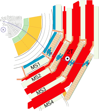
While uons can be reconstructed using only the muon system, the best measurements come from combining information from the muon detectors and the tracking detectors. Muons that leave clear signals in both of these detectors are called “global muons”. Muons have many features in common with electrons, but their own unique identification algorithms. We will use the same NanoAOD file as in the previous episode to look at the Muon NanoAOD branches.
| Object property | Type | Description |
|---|---|---|
| Muon_charge | Int_t | electric charge |
| Muon_cleanmask | UChar_t | simple cleaning mask with priority to leptons |
| Muon_dxy | Float_t | dxy (with sign) wrt first PV, in cm |
| Muon_dxyErr | Float_t | dxy uncertainty, in cm |
| Muon_dxybs | Float_t | dxy (with sign) wrt the beam spot, in cm |
| Muon_dz | Float_t | dz (with sign) wrt first PV, in cm |
| Muon_dzErr | Float_t | dz uncertainty, in cm |
| Muon_eta | Float_t | eta |
| Muon_fsrPhotonIdx | Int_t | (index to Fsrphoton) Index of the associated FSR photon |
| Muon_highPtId | UChar_t | high-pT cut-based ID (1 = tracker high pT, 2 = global high pT, which includes tracker high pT) |
| Muon_highPurity | Bool_t | inner track is high purity |
| Muon_inTimeMuon | Bool_t | inTimeMuon ID |
| Muon_ip3d | Float_t | 3D impact parameter wrt first PV, in cm |
| Muon_isGlobal | Bool_t | muon is global muon |
| Muon_isPFcand | Bool_t | muon is PF candidate |
| Muon_isStandalone | Bool_t | muon is a standalone muon |
| Muon_isTracker | Bool_t | muon is tracker muon |
| Muon_jetIdx | Int_t | (index to Jet) index of the associated jet (-1 if none) |
| Muon_jetNDauCharged | UChar_t | number of charged daughters of the closest jet |
| Muon_jetPtRelv2 | Float_t | Relative momentum of the lepton with respect to the closest jet after subtracting the lepton |
| Muon_jetRelIso | Float_t | Relative isolation in matched jet (1/ptRatio-1, pfRelIso04_all if no matched jet) |
| Muon_looseId | Bool_t | muon is loose muon |
| Muon_mass | Float_t | mass |
| Muon_mediumId | Bool_t | cut-based ID, medium WP |
| Muon_mediumPromptId | Bool_t | cut-based ID, medium prompt WP |
| Muon_miniIsoId | UChar_t | MiniIso ID from miniAOD selector (1=MiniIsoLoose, 2=MiniIsoMedium, 3=MiniIsoTight, 4=MiniIsoVeryTight) |
| Muon_miniPFRelIso_all | Float_t | mini PF relative isolation, total (with scaled rho*EA PU corrections) |
| Muon_miniPFRelIso_chg | Float_t | mini PF relative isolation, charged component |
| Muon_multiIsoId | UChar_t | MultiIsoId from miniAOD selector (1=MultiIsoLoose, 2=MultiIsoMedium) |
| Muon_mvaId | UChar_t | Mva ID from miniAOD selector (1=MvaLoose, 2=MvaMedium, 3=MvaTight, 4=MvaVTight, 5=MvaVVTight) |
| Muon_mvaLowPt | Float_t | Low pt muon ID score |
| Muon_mvaLowPtId | UChar_t | Low Pt Mva ID from miniAOD selector (1=LowPtMvaLoose, 2=LowPtMvaMedium) |
| Muon_mvaTTH | Float_t | TTH MVA lepton ID score |
| Muon_nStations | Int_t | number of matched stations with default arbitration (segment & track) |
| Muon_nTrackerLayers | Int_t | number of layers in the tracker |
| Muon_pdgId | Int_t | PDG code assigned by the event reconstruction (not by MC truth) |
| Muon_pfIsoId | UChar_t | PFIso ID from miniAOD selector (1=PFIsoVeryLoose, 2=PFIsoLoose, 3=PFIsoMedium, 4=PFIsoTight, 5=PFIsoVeryTight, 6=PFIsoVeryVeryTight) |
| Muon_pfRelIso03_all | Float_t | PF relative isolation dR=0.3, total (deltaBeta corrections) |
| Muon_pfRelIso03_chg | Float_t | PF relative isolation dR=0.3, charged component |
| Muon_pfRelIso04_all | Float_t | PF relative isolation dR=0.4, total (deltaBeta corrections) |
| Muon_phi | Float_t | phi |
| Muon_pt | Float_t | pt |
| Muon_ptErr | Float_t | ptError of the muon track |
| Muon_puppiIsoId | UChar_t | PuppiIsoId from miniAOD selector (1=Loose, 2=Medium, 3=Tight) |
| Muon_segmentComp | Float_t | muon segment compatibility |
| Muon_sip3d | Float_t | 3D impact parameter significance wrt first PV |
| Muon_softId | Bool_t | soft cut-based ID |
| Muon_softMva | Float_t | soft MVA ID score |
| Muon_softMvaId | Bool_t | soft MVA ID |
| Muon_tightCharge | Int_t | Tight charge criterion using pterr/pt of muonBestTrack (0:fail, 2:pass) |
| Muon_tightId | Bool_t | cut-based ID, tight WP |
| Muon_tkIsoId | UChar_t | TkIso ID (1=TkIsoLoose, 2=TkIsoTight) |
| Muon_tkRelIso | Float_t | Tracker-based relative isolation dR=0.3 for highPt, trkIso/tunePpt |
| Muon_triggerIdLoose | Bool_t | TriggerIdLoose ID |
| Muon_tunepRelPt | Float_t | TuneP relative pt, tunePpt/pt |
| nMuon | UInt_t | slimmedMuons after basic selection (pt > 15 |
Muon 4-vector and track-related variables
These branches for muons are very similar to those we saw earlier for electrons:
-
pt,eta,phi, andmassform the 4-vector -
chargeandtightChargegive electric charge information -
dxy,dz,ip3d, and their uncertainties or significances give impact parameter information
| Object property | Type | Description |
|---|---|---|
| Muon_charge | Int_t | electric charge |
| Muon_dxy | Float_t | dxy (with sign) wrt first PV, in cm |
| Muon_dxyErr | Float_t | dxy uncertainty, in cm |
| Muon_dxybs | Float_t | dxy (with sign) wrt the beam spot, in cm |
| Muon_dz | Float_t | dz (with sign) wrt first PV, in cm |
| Muon_dzErr | Float_t | dz uncertainty, in cm |
| Muon_eta | Float_t | eta |
| Muon_ip3d | Float_t | 3D impact parameter wrt first PV, in cm |
| Muon_mass | Float_t | mass |
| Muon_phi | Float_t | phi |
| Muon_pt | Float_t | pt |
| Muon_sip3d | Float_t | 3D impact parameter significance wrt first PV |
| Muon_tightCharge | Int_t | Tight charge criterion using pterr/pt of muonBestTrack (0:fail, 2:pass) |
Muon identification and isolation
The CMS Muon object group has several identification algorithms and
the pass/fail decisions for several working points are stored in
NanoAOD. A set of cut-based identification working points are available:
looseId, mediumId,
mediumPromptId, softId, highPtId.
Another set of identification algorithms are based on MVA discriminants:
mvaId, mvaLowPtId, mvaTTH,
softMvaId.
| Object property | Type | Description |
|---|---|---|
| Muon_highPtId | UChar_t | high-pT cut-based ID (1 = tracker high pT, 2 = global high pT, which includes tracker high pT) |
| Muon_looseId | Bool_t | muon is loose muon |
| Muon_mediumId | Bool_t | cut-based ID, medium WP |
| Muon_mediumPromptId | Bool_t | cut-based ID, medium prompt WP |
| Muon_mvaId | UChar_t | Mva ID from miniAOD selector (1=MvaLoose, 2=MvaMedium, 3=MvaTight, 4=MvaVTight, 5=MvaVVTight) |
| Muon_mvaLowPtId | UChar_t | Low Pt Mva ID from miniAOD selector (1=LowPtMvaLoose, 2=LowPtMvaMedium) |
| Muon_mvaTTH | Float_t | TTH MVA lepton ID score |
| Muon_softId | Bool_t | soft cut-based ID |
| Muon_softMvaId | Bool_t | soft MVA ID |
| Muon_tightId | Bool_t | cut-based ID, tight WP |
Just as we discussed for electrons, muons that are produced right away during a collision are usually separated from the other objects in the event, or isolated. For instance, an isolated muon might be produced in the decay of a W boson. In contrast, a non-isolated muon might come from hadrons decaying inside a jet.
Muon isolation is calculated from a combination of factors: energy from charged hadrons, energy from neutral hadrons, and energy from photons, all in a cone around the muon. Two cone sizes are used: either radii of 0.3 or 0.4, measured in angular units. Many algorithms also feature a correction factor that subtracts average energy expected from extra simultaneous collisions to this cone. This energy sum is then divided by the muon’s transverse momentum to form “relative” isolation. The whole calculation looks like this:
\(I_{\mu} = \frac{1}{p_{T}} \sum_{R<0.4} \left( p_{T}^{\mathrm{charged\,hadrons}} + \max(p_{T}^{\mathrm{photons}} + p_{T}^{\mathrm{neutral\,hadrons}} - \beta p_{T}^{\mathrm{charged\,pileup}} , 0) \right)\)
Many forms of muon isolation are stored in NanoAOD, as shown in the
table. The primary particle-flow isolation variable is
Muon_pfIsoId. Another type of isolation in common us is
“mini”-isolation, Muon_miniIsoId, which adapts the size of
the cone to improve efficiency for leptons that might exist near jets
because they were decay products of a high-momentum particle, such as a
top quark.
| Object property | Type | Description |
|---|---|---|
| Muon_jetRelIso | Float_t | Relative isolation in matched jet (1/ptRatio-1, pfRelIso04_all if no matched jet) |
| Muon_miniIsoId | UChar_t | MiniIso ID from miniAOD selector (1=MiniIsoLoose, 2=MiniIsoMedium, 3=MiniIsoTight, 4=MiniIsoVeryTight) |
| Muon_miniPFRelIso_all | Float_t | mini PF relative isolation, total (with scaled rho*EA PU corrections) |
| Muon_miniPFRelIso_chg | Float_t | mini PF relative isolation, charged component |
| Muon_multiIsoId | UChar_t | MultiIsoId from miniAOD selector (1=MultiIsoLoose, 2=MultiIsoMedium) |
| Muon_pfIsoId | UChar_t | PFIso ID from miniAOD selector (1=PFIsoVeryLoose, 2=PFIsoLoose, 3=PFIsoMedium, 4=PFIsoTight, 5=PFIsoVeryTight, 6=PFIsoVeryVeryTight) |
| Muon_pfRelIso03_all | Float_t | PF relative isolation dR=0.3, total (deltaBeta corrections) |
| Muon_pfRelIso03_chg | Float_t | PF relative isolation dR=0.3, charged component |
| Muon_pfRelIso04_all | Float_t | PF relative isolation dR=0.4, total (deltaBeta corrections) |
| Muon_puppiIsoId | UChar_t | PuppiIsoId from miniAOD selector (1=Loose, 2=Medium, 3=Tight) |
| Muon_tkIsoId | UChar_t | TkIso ID (1=TkIsoLoose, 2=TkIsoTight) |
| Muon_tkRelIso | Float_t | Tracker-based relative isolation dR=0.3 for highPt, trkIso/tunePpt |
Muon cross-reference indices
Like electrons, muons can be cross-referenced to other arrays in the NanoAOD file:
| Object property | Type | Description |
|---|---|---|
| Muon_fsrPhotonIdx | Int_t | (index to Fsrphoton) Index of the associated FSR photon |
| Muon_jetIdx | Int_t | (index to Jet) index of the associated jet (-1 if none) |
Tau leptons
The CMS Tau object group relies almost entirely on pre-computed algorithms to determine the quality of the tau reconstruction and the decay type. Since this object is not stable and has several decay modes, different combinations of identification and isolation algorithms are used across different analyses. The Run 1 Tau ID page and Nutshell Recipe provide a large table of algorithms that remains a valuable reference.
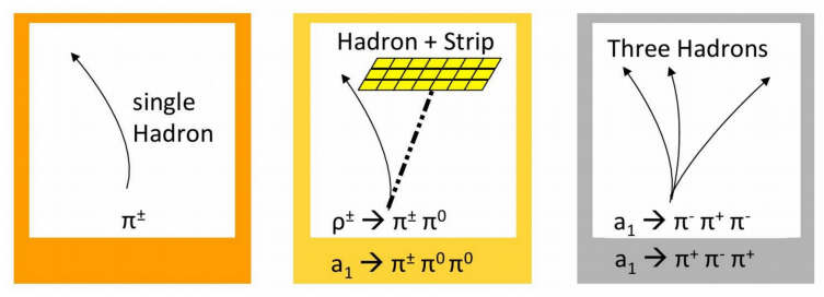
Taus that decay to leptons are typically identified as electrons or muons in CMS. But taus that decay to hadrons can be identified in the calorimeters based on the characteristic size and shape of their clusters.
| Object property | Type | Description |
|---|---|---|
| Tau_charge | Int_t | electric charge |
| Tau_chargedIso | Float_t | charged isolation |
| Tau_cleanmask | UChar_t | simple cleaning mask with priority to leptons |
| Tau_decayMode | Int_t | decayMode() |
| Tau_dxy | Float_t | d_{xy} of lead track with respect to PV, in cm (with sign) |
| Tau_dz | Float_t | d_{z} of lead track with respect to PV, in cm (with sign) |
| Tau_eta | Float_t | eta |
| Tau_idAntiEleDeadECal | Bool_t | Anti-electron dead-ECal discriminator |
| Tau_idAntiMu | UChar_t | Anti-muon discriminator V3: : bitmask 1 = Loose, 2 = Tight |
| Tau_idDecayModeOldDMs | Bool_t | tauID(‘decayModeFinding’) |
| Tau_idDeepTau2017v2p1VSe | UChar_t | byDeepTau2017v2p1VSe ID working points (deepTau2017v2p1): bitmask 1 = VVVLoose, 2 = VVLoose, 4 = VLoose, 8 = Loose, 16 = Medium, 32 = Tight, 64 = VTight, 128 = VVTight |
| Tau_idDeepTau2017v2p1VSjet | UChar_t | byDeepTau2017v2p1VSjet ID working points (deepTau2017v2p1): bitmask 1 = VVVLoose, 2 = VVLoose, 4 = VLoose, 8 = Loose, 16 = Medium, 32 = Tight, 64 = VTight, 128 = VVTight |
| Tau_idDeepTau2017v2p1VSmu | UChar_t | byDeepTau2017v2p1VSmu ID working points (deepTau2017v2p1): bitmask 1 = VLoose, 2 = Loose, 4 = Medium, 8 = Tight |
| Tau_jetIdx | Int_t | (index to Jet) index of the associated jet (-1 if none) |
| Tau_leadTkDeltaEta | Float_t | eta of the leading track, minus tau eta |
| Tau_leadTkDeltaPhi | Float_t | phi of the leading track, minus tau phi |
| Tau_leadTkPtOverTauPt | Float_t | pt of the leading track divided by tau pt |
| Tau_mass | Float_t | mass |
| Tau_neutralIso | Float_t | neutral (photon) isolation |
| Tau_phi | Float_t | phi |
| Tau_photonsOutsideSignalCone | Float_t | sum of photons outside signal cone |
| Tau_pt | Float_t | pt |
| Tau_puCorr | Float_t | pileup correction |
| Tau_rawDeepTau2017v2p1VSe | Float_t | byDeepTau2017v2p1VSe raw output discriminator (deepTau2017v2p1) |
| Tau_rawDeepTau2017v2p1VSjet | Float_t | byDeepTau2017v2p1VSjet raw output discriminator (deepTau2017v2p1) |
| Tau_rawDeepTau2017v2p1VSmu | Float_t | byDeepTau2017v2p1VSmu raw output discriminator (deepTau2017v2p1) |
| Tau_rawIso | Float_t | combined isolation (deltaBeta corrections) |
| Tau_rawIsodR03 | Float_t | combined isolation (deltaBeta corrections, dR=0.3) |
| nTau | UInt_t | slimmedTaus after basic selection (pt > 18 && tauID(‘decayModeFindingNewDMs’) && (tauID(‘byLooseCombinedIsolationDeltaBetaCorr3Hits’) |
Tau identification variables
The following variables in the tau collection represent the identification and isolation variables.
| Object property | Type | Description |
|---|---|---|
| Tau_decayMode | Int_t | decayMode() |
| Tau_idAntiEleDeadECal | Bool_t | Anti-electron dead-ECal discriminator |
| Tau_idAntiMu | UChar_t | Anti-muon discriminator V3: : bitmask 1 = Loose, 2 = Tight |
| Tau_idDecayModeOldDMs | Bool_t | tauID(‘decayModeFinding’) |
| Tau_idDeepTau2017v2p1VSe | UChar_t | byDeepTau2017v2p1VSe ID working points (deepTau2017v2p1): bitmask 1 = VVVLoose, 2 = VVLoose, 4 = VLoose, 8 = Loose, 16 = Medium, 32 = Tight, 64 = VTight, 128 = VVTight |
| Tau_idDeepTau2017v2p1VSjet | UChar_t | byDeepTau2017v2p1VSjet ID working points (deepTau2017v2p1): bitmask 1 = VVVLoose, 2 = VVLoose, 4 = VLoose, 8 = Loose, 16 = Medium, 32 = Tight, 64 = VTight, 128 = VVTight |
| Tau_idDeepTau2017v2p1VSmu | UChar_t | byDeepTau2017v2p1VSmu ID working points (deepTau2017v2p1): bitmask 1 = VLoose, 2 = Loose, 4 = Medium, 8 = Tight |
| Tau_rawIso | Float_t | combined isolation (deltaBeta corrections) |
| Tau_rawIsodR03 | Float_t | combined isolation (deltaBeta corrections, dR=0.3) |
Other tau information
Information about the tau lepton 4-vectors, cross-reference indices, impact parameters, etc, are analogous to the variables for electrons and muons.
- Track access may differ, but track-related member functions are common across objects.
- Physics objects in CMS are reconstructed from detector signals and are never 100% certain!
- Muons typically use pre-configured identification and isolation variables”
Content from Jets and MET
Last updated on 2026-07-16 | Edit this page
Estimated time: 15 minutes
Overview
Questions
- How are jets and missing transverse energy treated in CMS Open Data?
Objectives
- Identify jet and MET code collections in AOD files
- Understand typical features of jet/MET objects
After tracks and energy deposits in the CMS tracking detectors, calorimeters, and muon detectors are reconstructed as particle flow candidates, an event can be interpreted in various ways. Two common elements of event interpretation are clustering jets and calculating missing transverse momentum.
Jets
When a quark or gluon travels through the detector material, it creates a dense shower of long-lived particles. These particles can be clustered together into “jets”. The momentum and energy of a jet resembles that of the initial quark or gluon that produced it. In the CMS language, jets are made up of many particles, with the following predictable energy composition:
- ~65% charged hadrons
- ~25% photons (usually produced when neutral pi mesons decay)
- ~10% neutral hadrons
Jets are very messy! Hadron showers can produce 100s of particles near each other in the CMS detector, so these particles are rarely analyzed individually. How can we determine which particle candidates should be included in each jet?
Clustering
Jets can be clustered using a variety of different inputs from the CMS detector. “CaloJets” use only calorimeter energy deposits. “GenJets” use generated particles from a simulation. But by far the most common are “PFJets”, from particle flow candidates.
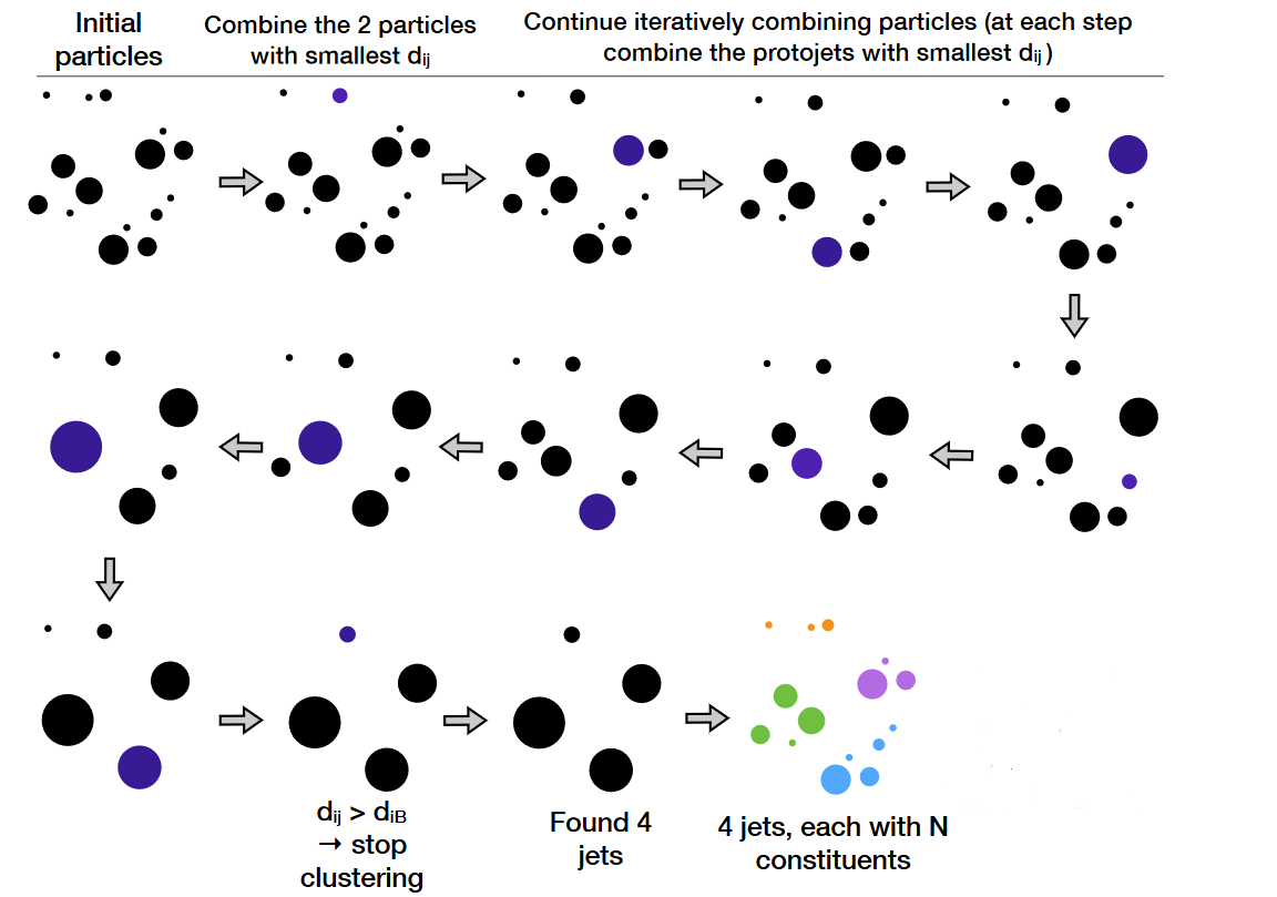
As we’ve learned, the result of the CMS Particle Flow algorithm is a list of particle candidates. These particles are formed into jets using a “clustering algorithm”. The most common algorithm used by CMS is the “anti-kt” algorithm, which is abbreviated “AK”. It iterates over particle pairs and finds the two (i and j) that are the closest in some distance measure and determines whether to combine them:
\(d_{ij} = \min(p^{-2}_{T,i},p^{-2}_{T,j}) \Delta R^2_{ij}/R^2\)
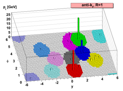
Particle pairs are combined as long as \(d_{ij} < p^{-2}_{T,i}\). The momentum power (-2) used by the anti-kt algorithm means that higher-momentum particles are clustered first. This leads to jets with a round shape that tend to be centered on the highest momentum particle.
Pileup
Inevitably, the list of particle flow candidates contains particles that did not originate from the primary collision. CMS experiences multiple simultaneous collisions, called “pileup”, during each “bunch crossing” of the LHC, so particles from multiple collisions coexist in the detector. There are various methods to remove their contributions from jets:
- Charged hadron subtraction CHS: all charged hadron PF candidates are associated with a track. If the track is not connected with the primary vertex, that charged hadron can be removed from the list. CHS is limited to the region of the detector covered by the inner tracker. The pileup contribution to neutral hadrons has to be removed mathematically since those candidates have no tracks.
- PileUp Per Particle Identification (PUPPI, available in Run 2): CHS is applied, and then all remaining particles are weighted based on their likelihood of arising from pileup. This method is more stable and performs very well in high pileup scenarios such as the upcoming HL-LHC era.
Small-radius jets in NanoAOD
The most basic setting for anti-kt particle-flow jets in CMS is a radius parameter of 0.4. These jets are often called “AK4 jets” or “small-radius jets”. Their information is stored in the “Jet_*” collection in NanoAOD:
| Object property | Type | Description |
|---|---|---|
| Jet_area | Float_t | jet catchment area, for JECs |
| Jet_bRegCorr | Float_t | pt correction for b-jet energy regression |
| Jet_bRegRes | Float_t | res on pt corrected with b-jet regression |
| Jet_btagCSVV2 | Float_t | pfCombinedInclusiveSecondaryVertexV2 b-tag discriminator (aka CSVV2) |
| Jet_btagDeepB | Float_t | DeepCSV b+bb tag discriminator |
| Jet_btagDeepCvB | Float_t | DeepCSV c vs b+bb discriminator |
| Jet_btagDeepCvL | Float_t | DeepCSV c vs udsg discriminator |
| Jet_btagDeepFlavB | Float_t | DeepJet b+bb+lepb tag discriminator |
| Jet_btagDeepFlavCvB | Float_t | DeepJet c vs b+bb+lepb discriminator |
| Jet_btagDeepFlavCvL | Float_t | DeepJet c vs uds+g discriminator |
| Jet_btagDeepFlavQG | Float_t | DeepJet g vs uds discriminator |
| Jet_cRegCorr | Float_t | pt correction for c-jet energy regression |
| Jet_cRegRes | Float_t | res on pt corrected with c-jet regression |
| Jet_chEmEF | Float_t | charged Electromagnetic Energy Fraction |
| Jet_chFPV0EF | Float_t | charged fromPV==0 Energy Fraction (energy excluded from CHS jets). Previously called betastar. |
| Jet_chHEF | Float_t | charged Hadron Energy Fraction |
| Jet_cleanmask | UChar_t | simple cleaning mask with priority to leptons |
| Jet_electronIdx1 | Int_t | (index to Electron) index of first matching electron |
| Jet_electronIdx2 | Int_t | (index to Electron) index of second matching electron |
| Jet_eta | Float_t | eta |
| Jet_hfadjacentEtaStripsSize | Int_t | eta size of the strips next to the central tower strip in HF (noise discriminating variable) |
| Jet_hfcentralEtaStripSize | Int_t | eta size of the central tower strip in HF (noise discriminating variable) |
| Jet_hfsigmaEtaEta | Float_t | sigmaEtaEta for HF jets (noise discriminating variable) |
| Jet_hfsigmaPhiPhi | Float_t | sigmaPhiPhi for HF jets (noise discriminating variable) |
| Jet_jetId | Int_t | Jet ID flags bit1 is loose (always false in 2017 since it does not exist), bit2 is tight, bit3 is tightLepVeto |
| Jet_mass | Float_t | mass |
| Jet_muEF | Float_t | muon Energy Fraction |
| Jet_muonIdx1 | Int_t | (index to Muon) index of first matching muon |
| Jet_muonIdx2 | Int_t | (index to Muon) index of second matching muon |
| Jet_muonSubtrFactor | Float_t | 1-(muon-subtracted raw pt)/(raw pt) |
| Jet_nConstituents | UChar_t | Number of particles in the jet |
| Jet_nElectrons | Int_t | number of electrons in the jet |
| Jet_nMuons | Int_t | number of muons in the jet |
| Jet_neEmEF | Float_t | neutral Electromagnetic Energy Fraction |
| Jet_neHEF | Float_t | neutral Hadron Energy Fraction |
| Jet_phi | Float_t | phi |
| Jet_pt | Float_t | pt |
| Jet_puId | Int_t | Pileup ID flags with 106X (2016) training |
| Jet_puIdDisc | Float_t | Pileup ID discriminant with 106X (2016) training |
| Jet_qgl | Float_t | Quark vs Gluon likelihood discriminator |
| Jet_rawFactor | Float_t | 1 - Factor to get back to raw pT |
| nJet | UInt_t | slimmedJets, i.e. ak4 PFJets CHS with JECs applied, after basic selection (pt > 15) |
By now you should be able to identify the 4-vector information and the cross-reference indices in this list of branches! Many of the variables in the list will be discussed in the later lesson pages on heavy flavor tagging and jet energy corrections.
Jet identification
Particle-flow jets are not immune to noise in the detector, and jets used in analyses should be filtered to remove noise jets. CMS has defined a “noise jet ID” that considers information about the energy types within the jet:
- charged hadron fraction – what fraction of the jet consists of charged hadrons? This will be greater than 0 if the jet is within the inner tracker region.
- neutral hadron fraction – what fraction of the jet consists of neutral hadrons? This should always be less than 1.
- charged electromagnetic fraction – what fraction of the jet consists of electrons? This should always be less than 1.
- neutral electromagnetic fraction – what fraction of the jet consists of photons? This should always be less than 1.
- number of constituents – this should be greater than 1.
These criteria demonstrate how particle-flow jets combine information
across subdetectors. Jets will typically have energy from electrons and
photons, but those fractions of the total energy should be less than
one. Similarly, jets should have some energy from charged hadrons if
they overlap the inner tracker, and all the energy should not come from
neutral hadrons. A mixture of energy sources is expected for genuine
jets. All of these energy fractions (and more) can be accessed in
NanoAOD. Whenever you use jets, requirements should be placed on the
value of Jet_jetId, rejecting at least values of 0.
| Object property | Type | Description |
|---|---|---|
| Jet_chEmEF | Float_t | charged Electromagnetic Energy Fraction |
| Jet_chFPV0EF | Float_t | charged fromPV==0 Energy Fraction (energy excluded from CHS jets). Previously called betastar. |
| Jet_chHEF | Float_t | charged Hadron Energy Fraction |
| Jet_jetId | Int_t | Jet ID flags bit1 is loose (always false in 2017 since it does not exist), bit2 is tight, bit3 is tightLepVeto |
| Jet_muEF | Float_t | muon Energy Fraction |
| Jet_nConstituents | UChar_t | Number of particles in the jet |
| Jet_nElectrons | Int_t | number of electrons in the jet |
| Jet_nMuons | Int_t | number of muons in the jet |
| Jet_neEmEF | Float_t | neutral Electromagnetic Energy Fraction |
| Jet_neHEF | Float_t | neutral Hadron Energy Fraction |
| Jet_puId | Int_t | Pileup ID flags with 106X (2016) training |
Another important identification algorithm is the “pileup jet ID”, which can identify jets that are not likely to come from the primary collision of an event.
Large-radius jets in NanoAOD
Another useful anti-kt jet radius is 0.8, called “AK8 jets” or “large-radius jets”. These jets are stored if they have transverse momentum above 170 GeV, and are represented by the “FatJet_*” collection in NanoAOD:
| Object property | Type | Description |
|---|---|---|
| FatJet_area | Float_t | jet catchment area, for JECs |
| FatJet_btagCSVV2 | Float_t | pfCombinedInclusiveSecondaryVertexV2 b-tag discriminator (aka CSVV2) |
| FatJet_btagDDBvLV2 | Float_t | DeepDoubleX V2(mass-decorrelated) discriminator for H(Z)->bb vs QCD |
| FatJet_btagDDCvBV2 | Float_t | DeepDoubleX V2 (mass-decorrelated) discriminator for H(Z)->cc vs H(Z)->bb |
| FatJet_btagDDCvLV2 | Float_t | DeepDoubleX V2 (mass-decorrelated) discriminator for H(Z)->cc vs QCD |
| FatJet_btagDeepB | Float_t | DeepCSV b+bb tag discriminator |
| FatJet_btagHbb | Float_t | Higgs to BB tagger discriminator |
| FatJet_deepTagMD_H4qvsQCD | Float_t | Mass-decorrelated DeepBoostedJet tagger H->4q vs QCD discriminator |
| FatJet_deepTagMD_HbbvsQCD | Float_t | Mass-decorrelated DeepBoostedJet tagger H->bb vs QCD discriminator |
| FatJet_deepTagMD_TvsQCD | Float_t | Mass-decorrelated DeepBoostedJet tagger top vs QCD discriminator |
| FatJet_deepTagMD_WvsQCD | Float_t | Mass-decorrelated DeepBoostedJet tagger W vs QCD discriminator |
| FatJet_deepTagMD_ZHbbvsQCD | Float_t | Mass-decorrelated DeepBoostedJet tagger Z/H->bb vs QCD discriminator |
| FatJet_deepTagMD_ZHccvsQCD | Float_t | Mass-decorrelated DeepBoostedJet tagger Z/H->cc vs QCD discriminator |
| FatJet_deepTagMD_ZbbvsQCD | Float_t | Mass-decorrelated DeepBoostedJet tagger Z->bb vs QCD discriminator |
| FatJet_deepTagMD_ZvsQCD | Float_t | Mass-decorrelated DeepBoostedJet tagger Z vs QCD discriminator |
| FatJet_deepTagMD_bbvsLight | Float_t | Mass-decorrelated DeepBoostedJet tagger Z/H/gluon->bb vs light flavour discriminator |
| FatJet_deepTagMD_ccvsLight | Float_t | Mass-decorrelated DeepBoostedJet tagger Z/H/gluon->cc vs light flavour discriminator |
| FatJet_deepTag_H | Float_t | DeepBoostedJet tagger H(bb,cc,4q) sum |
| FatJet_deepTag_QCD | Float_t | DeepBoostedJet tagger QCD(bb,cc,b,c,others) sum |
| FatJet_deepTag_QCDothers | Float_t | DeepBoostedJet tagger QCDothers value |
| FatJet_deepTag_TvsQCD | Float_t | DeepBoostedJet tagger top vs QCD discriminator |
| FatJet_deepTag_WvsQCD | Float_t | DeepBoostedJet tagger W vs QCD discriminator |
| FatJet_deepTag_ZvsQCD | Float_t | DeepBoostedJet tagger Z vs QCD discriminator |
| FatJet_electronIdx3SJ | Int_t | (index to Electron) index of electron matched to jet |
| FatJet_eta | Float_t | eta |
| FatJet_jetId | Int_t | Jet ID flags bit1 is loose (always false in 2017 since it does not exist), bit2 is tight, bit3 is tightLepVeto |
| FatJet_lsf3 | Float_t | Lepton Subjet Fraction (3 subjets) |
| FatJet_mass | Float_t | mass |
| FatJet_msoftdrop | Float_t | Corrected soft drop mass with PUPPI |
| FatJet_muonIdx3SJ | Int_t | (index to Muon) index of muon matched to jet |
| FatJet_n2b1 | Float_t | N2 with beta=1 |
| FatJet_n3b1 | Float_t | N3 with beta=1 |
| FatJet_nConstituents | UChar_t | Number of particles in the jet |
| FatJet_particleNetMD_QCD | Float_t | Mass-decorrelated ParticleNet tagger raw QCD score |
| FatJet_particleNetMD_Xbb | Float_t | Mass-decorrelated ParticleNet tagger raw X->bb score. For X->bb vs QCD tagging, use Xbb/(Xbb+QCD) |
| FatJet_particleNetMD_Xcc | Float_t | Mass-decorrelated ParticleNet tagger raw X->cc score. For X->cc vs QCD tagging, use Xcc/(Xcc+QCD) |
| FatJet_particleNetMD_Xqq | Float_t | Mass-decorrelated ParticleNet tagger raw X->qq (uds) score. For X->qq vs QCD tagging, use Xqq/(Xqq+QCD). For W vs QCD tagging, use (Xcc+Xqq)/(Xcc+Xqq+QCD) |
| FatJet_particleNet_H4qvsQCD | Float_t | ParticleNet tagger H(->VV->qqqq) vs QCD discriminator |
| FatJet_particleNet_HbbvsQCD | Float_t | ParticleNet tagger H(->bb) vs QCD discriminator |
| FatJet_particleNet_HccvsQCD | Float_t | ParticleNet tagger H(->cc) vs QCD discriminator |
| FatJet_particleNet_QCD | Float_t | ParticleNet tagger QCD(bb,cc,b,c,others) sum |
| FatJet_particleNet_TvsQCD | Float_t | ParticleNet tagger top vs QCD discriminator |
| FatJet_particleNet_WvsQCD | Float_t | ParticleNet tagger W vs QCD discriminator |
| FatJet_particleNet_ZvsQCD | Float_t | ParticleNet tagger Z vs QCD discriminator |
| FatJet_particleNet_mass | Float_t | ParticleNet mass regression |
| FatJet_phi | Float_t | phi |
| FatJet_pt | Float_t | pt |
| FatJet_rawFactor | Float_t | 1 - Factor to get back to raw pT |
| FatJet_subJetIdx1 | Int_t | (index to Subjet) index of first subjet |
| FatJet_subJetIdx2 | Int_t | (index to Subjet) index of second subjet |
| FatJet_tau1 | Float_t | Nsubjettiness (1 axis) |
| FatJet_tau2 | Float_t | Nsubjettiness (2 axis) |
| FatJet_tau3 | Float_t | Nsubjettiness (3 axis) |
| FatJet_tau4 | Float_t | Nsubjettiness (4 axis) |
| nFatJet | UInt_t | slimmedJetsAK8, i.e. ak8 fat jets for boosted analysis |
Beyond the 4-vector information, FatJet_jetId variable,
and cross-reference indices, the overwhelming majority of variables
stored for FatJets are used to identify hadronic decays of high-momentum
massive SM particles like top quarks, Higgs bosons, W bosons, and Z
bosons. This will be covered in the next page.
MET
Missing transverse momentum is the negative vector sum of the transverse momenta of all particle flow candidates in an event. The magnitude of the missing transverse momentum vector is called missing transverse energy and referred to with the acronym “MET”. In a perfect collision, the colliding particles would have exactly 0 momentum in the \(x\) or \(y\) direction. If all of the collision products are detecter perfectly in CMS, the “missing” momentum found when we calculate this vector sum would also be 0. In real life, some particles are not detected at all by CMS, and all particles are measured with slight imperfections, creating MET. Types of particles that would produce “real” MET include neutrinos, dark matter particles, or other exotic particles that would not interact in CMS.
| Object property | Type | Description |
|---|---|---|
| MET_phi | Float_t | phi |
| MET_pt | Float_t | pt |
| MET_significance | Float_t | MET significance |
| MET_sumEt | Float_t | scalar sum of Et |
| MET_sumPtUnclustered | Float_t | sumPt used for MET significance |
The standard “MET” magnitude is found in MET_pt, and the
azimuthal angle of the vector is MET_phi (since MET can
only be computed in the transverse plane, no MET_eta is
found). The MET_significance variable can be a useful tool:
it describes the likelihood that the MET arose from noise or
mismeasurement in the detector as opposed to a neutrino or similar
non-interacting particle. The four-vectors of the other physics objects
along with their uncertainties are required to compute the significance
of the MET signature. MET that is directed nearly (anti)colinnear with a
physics object is likely to arise from mismeasurement and should not
have a large significance.
- Jets are spatially-grouped collections of particles that traversed the CMS detector
- Particles from additional proton-proton collisions (pileup) must be removed from jets
- Missing transverse energy is the negative vector sum of particle candidates
- Many of the variables discussed for other objects also exist for jets
Content from Jet flavor tagging
Last updated on 2026-07-16 | Edit this page
Estimated time: 20 minutes
Overview
Questions
- How are b hadrons identified in CMS?
- How are the parent particles of large-radius jets identified in CMS?
Objectives
- Understand the basics of heavy flavor tagging
- Learn to access tagging information in NanoAOD files
Jet reconstruction and identification is an important part of the
analyses at the LHC. Jets can originate from many different types of
particles. The figure below gives an example of how different “parent
particles” can influence the internal structure of a jet. Observables
related to the mass and internal
structure of a jet can help us design algorithms to distinguish
between sources. 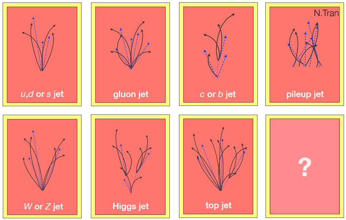
Several “b tagging” algorithms exist to identify jets from b quarks, which have unique properties that distinguish them from light quark or gluon jets.
B Tagging Algorithms
Tagging algorithms first connect jets with particle tracks that are either connected to one of the jet’s particle flow candidates, or lie within a nearby cone. Both tracks and “secondary vertices” (points where multiple tracks emerge within a jet) can be used in track-based, vertex-based, or “combined” tagging algorithms. The specific details depend upon the algorithm, but they all rely on special properties of b hadrons such as:
- long lifetime compared to other particles produced in a collision, which allows b hadrons to travel away from the collision before decaying,
- large mass,
- high number of tracks compared to other types of quark jets,
- higher probability of producing a low-momentum electron or muon.
In recent CMS Open Data, the most important b-tagging algorithms are:
- Combined Secondary Vertex (CSV): many properties of jets, tracks, and secondary vertices are combined into a “boosted decision tree”, which is a simple form of machine learning. This tagger became the default CMS algorithm in Run 1 and early Run 2.
- DeepCSV: the CSV algorithm was reimagined as a deep neural network.
- DeepJet: this deep neural network tagger uses a more complex architecture than DeepCSV, and is the most powerful b tagging algorithm for Run 2.
These algorithms produce a single, real number called a b tagging “discriminator” for each jet. The more positive the discriminator value, the more likely it is that this jet contained b hadrons. The DeepCSV and DeepJet algorithms can also identify charm-flavor jets, and DeepJet can even distinguish between light-quark and gluon jets.
| Object property | Type | Description |
|---|---|---|
| Jet_btagCSVV2 | Float_t | pfCombinedInclusiveSecondaryVertexV2 b-tag discriminator (aka CSVV2) |
| Jet_btagDeepB | Float_t | DeepCSV b+bb tag discriminator |
| Jet_btagDeepCvB | Float_t | DeepCSV c vs b+bb discriminator |
| Jet_btagDeepCvL | Float_t | DeepCSV c vs udsg discriminator |
| Jet_btagDeepFlavB | Float_t | DeepJet b+bb+lepb tag discriminator |
| Jet_btagDeepFlavCvB | Float_t | DeepJet c vs b+bb+lepb discriminator |
| Jet_btagDeepFlavCvL | Float_t | DeepJet c vs uds+g discriminator |
| Jet_btagDeepFlavQG | Float_t | DeepJet g vs uds discriminator |
Working points
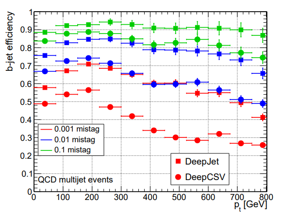
A jet is considered “b tagged” if the discriminator value exceeds some threshold. Different thresholds will have different efficiencies for identifying true b quark jets and for mis-tagging light quark jets. As we saw for muons and other objects, a “loose” working point will allow the highest mis-tagging rate, while a “tight” working point will sacrifice some correct-tag efficiency in order to reduce mis-tagging. The DeepCSV and DeepJet algorithms are supported by CMS for 2016 Open Data.
The supported working points for DeepCSV and DeepJet for the 2016 Open Data are:
- Loose (10% misidentification rate):
Jet_btagDeepB> 0.1918 ,Jet_btagDeepFlav> 0.0480 - Medium (1% misidentification rate):
Jet_btagDeepB> 0.5847,Jet_btagDeepFlav> 0.2489 - Tight (0.1% misidentification rate):
Jet_btagDeepB> 0.8767,Jet_btagDeepFlav> 0.6377
The figure below shows the relationship between b jet efficiency and working point in DeepCSV and DeepJet:
FatJet tagging algorithms
In CMS NanoAOD, the “fat” jets have a larger cone size than standard jets. These larger jets are ideal for identifying top quarks or W, Z, or Higgs bosons that have been produced with high momentum and have decayed to several quarks. All of these decay products can be caught within one large-radius jet cone. Several identification algorithms are used in CMS to tell the different sources apart.
Groomed mass and substructure
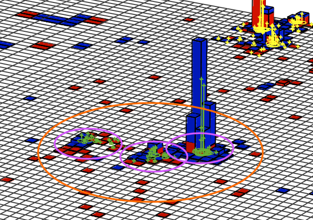
The mass of a jet is evaluated by summing the energy-momentum four-vectors of all the particle flow candidates that make up the jet and computing the mass of the resulting object. This mass calculation is distorted by gluons that radiate energy away from the initial particles that formed the jet. For example, the masses of light quark jets are measured to be much larger than the actual masses of these quarks – typically 10–50 GeV. Mass Grooming procedures can help reduce the impact of this radiation and bring the jet mass closer to the true values of the parent particles. Grooming algorithms typically cluster the jet’s consitituents into “subjets”, like those represented by the small circles in the figure below. The relationships between different subjets can then be tested to decide which to keep.
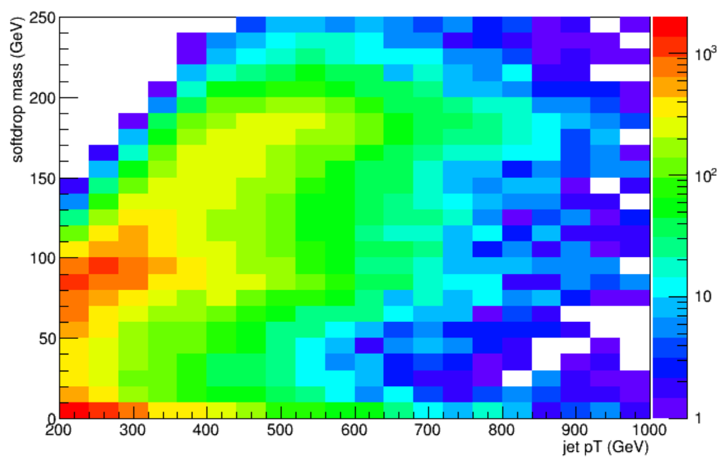
The “softdrop” mass is included in NanoAOD for large-radius jets. In the “softdrop” procedure, jets are recursively de-clustered, and at each step subjets that are too low in momentum or large angles separating them from other subjets are discarded. The following image shows the relationship between FatJet momentum, mass, and jet radius. As the momentum increases, jets of larger mass become contained within the FatJet. While W bosons with a mass of 80 GeV can be observed from 200 GeV, top quarks with a mass of 170 GeV require a higher momentum threshold.
The internal structure of a jet can be probed using many observables: N-subjettiness, energy correlation functions, and others. In CMS, N-subjettiness is the default jet substructure variable for identifying boosted particle decays.
The “tau” variables of N-subjettiness, defined below, are jet shape variables whose value approaches 0 for jets having N or fewer subjets. Top quarks typically decay to 3 quarks, so we would expect small tau values for N = 3, 4, 5, 6, etc, but larger values for N = 1 or 2.
\(\tau_{N} = \frac{\sum^{n_{\mathrm{constituents}}}_{i=1} p_{\mathrm{T},i} \min{\Delta R_{1,i}, \Delta R_{2,i}, \ldots, \Delta R_{N,i}}}{\sum^{n_{\mathrm{constituents}}}_{i=1} p_{T,i}R}\)
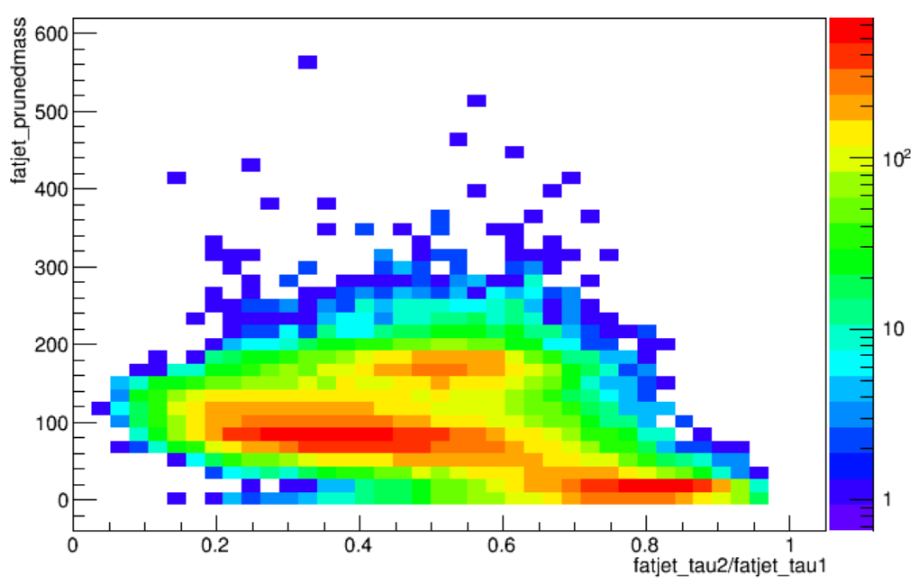
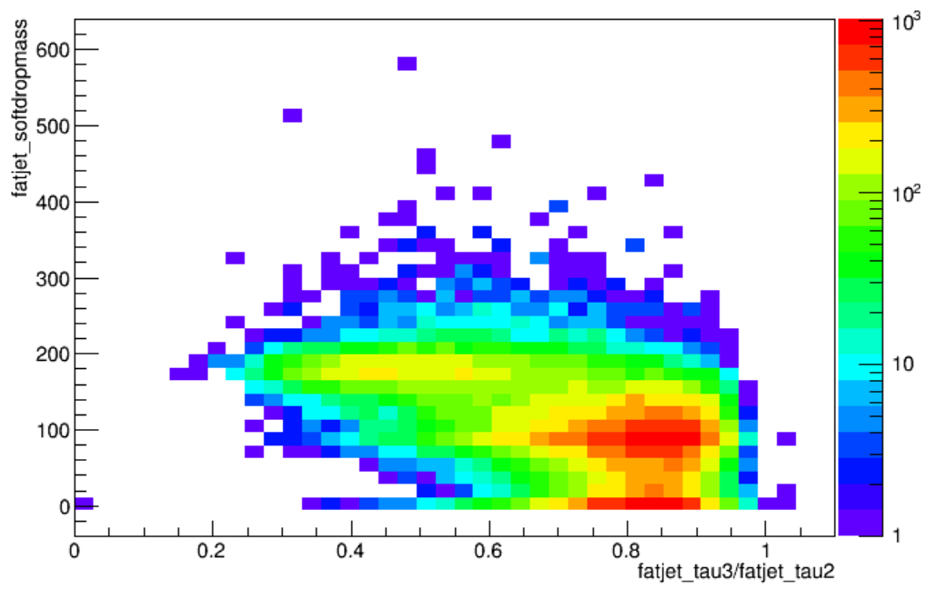
Ratios of tau values provide the best discrimination for jets with a specific number of subjets. For two-quark jets like W, Z, or H boson decays, we study the ratio tau_2 / tau_1. For three-quark jets we study tau_3 / tau_2.
The figures below show the relevant tau ratios for W boson (left) and top quark (right) jets. The structure in the tau_2/tau_1 plot is very unique: W bosons pool at lower values of tau_2/tau_1, while top quarks (with more than 2 subjets) and light quarks (with only 1 subjet) pool at medium and higher values. In the tau_3/tau_2 plot, top quark jets have low values while both W boson and light quark jets are gathered near 1.
 |
| 
For top quark or H boson decays, applying b tagging algorithms to the subjets of the large-radius jets gives another valuable substructure observable. The Combined Secondary Vertex v2 and the DeepCSV discriminants have been stored for the two subjets obtained from the soft drop algorithm in each large-radius jet. For simulation, we also store the generator-level flavor information for the subjet. You can explore the “Subjet” branches in NanoAOD here
Finally, NanoAOD contains some energy correlation function information for large-radius jets. The N2 and N3 functions are described in detail in a CMS paper on boosted jet identification.
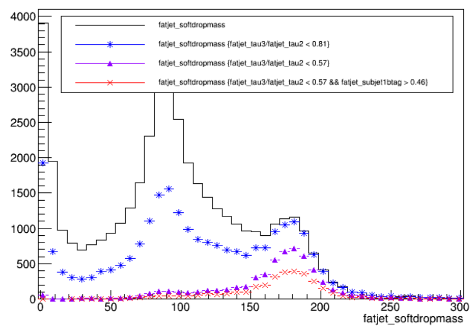
Groomed mass, jet substructure, and subjet b-tagging were the backbone of early boosted jet identification in CMS. The figure below shows an example of isolating top quark jets by applying various mass and substructure criteria. However, these algorithms have now been eclipsed by deep neural network identification techniques.
| Object property | Type | Description |
|---|---|---|
| FatJet_msoftdrop | Float_t | Corrected soft drop mass with PUPPI |
| FatJet_n2b1 | Float_t | N2 with beta=1 |
| FatJet_n3b1 | Float_t | N3 with beta=1 |
| FatJet_subJetIdx1 | Int_t | (index to Subjet) index of first subjet |
| FatJet_subJetIdx2 | Int_t | (index to Subjet) index of second subjet |
| FatJet_tau1 | Float_t | Nsubjettiness (1 axis) |
| FatJet_tau2 | Float_t | Nsubjettiness (2 axis) |
| FatJet_tau3 | Float_t | Nsubjettiness (3 axis) |
| FatJet_tau4 | Float_t | Nsubjettiness (4 axis) |
Deep Neural Network taggers
During Run 2, CMS analysts developed many neural network identification schemes for large-radius jets. The best performers have been preserved in the version of NanoAOD available for Open Data. The main algorithms are:
- DeepDoubleX (or “double-b”): a Boosted Decision Tree optimized for decays of massive particles to a pair of b or c quarks.
- DeepBoostedJet (or “DeepAK8”): a Convolutional Neural Network combined with a dense network that uses particle-flow candidates and secondary vertices to determine the parent particle of the jet
- ParticleNet: a Dynamic Graph Convolutional Neural Network applied on “point cloud” data structures built from the particle-flow candidates within a jet.
The deep network taggers provide discriminants for many different particle hypotheses. These are typically grouped into “binarized” discriminants intended to separate a particular massive particle (top, Higgs, etc) from light quark jets. Both DeepAK8 and ParticleNet offer “mass-decorrelated” discriminants, for which the network has been trained in such a way that jet mass is not part of the learning process. For analyses that use the jet mass distribution as a key sensitive variable, decorrelation helps maintain a smoothly falling light-quark jet mass distribution, with no artificial peak near the region of interest (eg, near 125 GeV for Higgs bosons, or new 170 GeV for top quarks).
The branches available in NanoAOD for the deep network taggers are listed below.
| Object property | Type | Description |
|---|---|---|
| FatJet_btagDDBvLV2 | Float_t | DeepDoubleX V2(mass-decorrelated) discriminator for H(Z)->bb vs QCD |
| FatJet_btagDDCvBV2 | Float_t | DeepDoubleX V2 (mass-decorrelated) discriminator for H(Z)->cc vs H(Z)->bb |
| FatJet_btagDDCvLV2 | Float_t | DeepDoubleX V2 (mass-decorrelated) discriminator for H(Z)->cc vs QCD |
| FatJet_btagHbb | Float_t | Higgs to BB tagger discriminator |
| FatJet_deepTagMD_H4qvsQCD | Float_t | Mass-decorrelated DeepBoostedJet tagger H->4q vs QCD discriminator |
| FatJet_deepTagMD_HbbvsQCD | Float_t | Mass-decorrelated DeepBoostedJet tagger H->bb vs QCD discriminator |
| FatJet_deepTagMD_TvsQCD | Float_t | Mass-decorrelated DeepBoostedJet tagger top vs QCD discriminator |
| FatJet_deepTagMD_WvsQCD | Float_t | Mass-decorrelated DeepBoostedJet tagger W vs QCD discriminator |
| FatJet_deepTagMD_ZHbbvsQCD | Float_t | Mass-decorrelated DeepBoostedJet tagger Z/H->bb vs QCD discriminator |
| FatJet_deepTagMD_ZHccvsQCD | Float_t | Mass-decorrelated DeepBoostedJet tagger Z/H->cc vs QCD discriminator |
| FatJet_deepTagMD_ZbbvsQCD | Float_t | Mass-decorrelated DeepBoostedJet tagger Z->bb vs QCD discriminator |
| FatJet_deepTagMD_ZvsQCD | Float_t | Mass-decorrelated DeepBoostedJet tagger Z vs QCD discriminator |
| FatJet_deepTagMD_bbvsLight | Float_t | Mass-decorrelated DeepBoostedJet tagger Z/H/gluon->bb vs light flavour discriminator |
| FatJet_deepTagMD_ccvsLight | Float_t | Mass-decorrelated DeepBoostedJet tagger Z/H/gluon->cc vs light flavour discriminator |
| FatJet_deepTag_H | Float_t | DeepBoostedJet tagger H(bb,cc,4q) sum |
| FatJet_deepTag_QCD | Float_t | DeepBoostedJet tagger QCD(bb,cc,b,c,others) sum |
| FatJet_deepTag_QCDothers | Float_t | DeepBoostedJet tagger QCDothers value |
| FatJet_deepTag_TvsQCD | Float_t | DeepBoostedJet tagger top vs QCD discriminator |
| FatJet_deepTag_WvsQCD | Float_t | DeepBoostedJet tagger W vs QCD discriminator |
| FatJet_deepTag_ZvsQCD | Float_t | DeepBoostedJet tagger Z vs QCD discriminator |
| FatJet_particleNetMD_QCD | Float_t | Mass-decorrelated ParticleNet tagger raw QCD score |
| FatJet_particleNetMD_Xbb | Float_t | Mass-decorrelated ParticleNet tagger raw X->bb score. For X->bb vs QCD tagging, use Xbb/(Xbb+QCD) |
| FatJet_particleNetMD_Xcc | Float_t | Mass-decorrelated ParticleNet tagger raw X->cc score. For X->cc vs QCD tagging, use Xcc/(Xcc+QCD) |
| FatJet_particleNetMD_Xqq | Float_t | Mass-decorrelated ParticleNet tagger raw X->qq (uds) score. For X->qq vs QCD tagging, use Xqq/(Xqq+QCD). For W vs QCD tagging, use (Xcc+Xqq)/(Xcc+Xqq+QCD) |
| FatJet_particleNet_H4qvsQCD | Float_t | ParticleNet tagger H(->VV->qqqq) vs QCD discriminator |
| FatJet_particleNet_HbbvsQCD | Float_t | ParticleNet tagger H(->bb) vs QCD discriminator |
| FatJet_particleNet_HccvsQCD | Float_t | ParticleNet tagger H(->cc) vs QCD discriminator |
| FatJet_particleNet_QCD | Float_t | ParticleNet tagger QCD(bb,cc,b,c,others) sum |
| FatJet_particleNet_TvsQCD | Float_t | ParticleNet tagger top vs QCD discriminator |
| FatJet_particleNet_WvsQCD | Float_t | ParticleNet tagger W vs QCD discriminator |
| FatJet_particleNet_ZvsQCD | Float_t | ParticleNet tagger Z vs QCD discriminator |
| FatJet_particleNet_mass | Float_t | ParticleNet mass regression |
- Tagging algorithms separate heavy flavor jets from jets produced by the hadronization of light quarks and gluons
- FatJet tagging algorithms can identify jets from massive SM particles
- Tagging algorithms produce a disriminator value for each jet that represents the likelihood that the jet came from a particular particle
- Each tagging algorithm has recommended ‘working points’ (discriminator values) based on a misidentification probability for non-interesting jets