Content from Introduction
Last updated on 2024-07-18 | Edit this page
Estimated time: 10 minutes
Overview
Questions
- What did we learn in the physics objects pre-learning module?
- How should I select events for a physics analysis?
Objectives
- Summarize information available for various physics objects.
- Describe the fundamental elements of event selection in CMS.
What we’ve learned so far…
The CMS experment is a giant detector that acts like a camera that “photographs” particle collisions, allowing us to interpret their nature. In the Physics Objects pre-learning exercise, you read about the following physics objects reconstructed by CMS:
- muons
- electrons
- photons
- taus
- jets
- missing transverse momentum
Many properties of these objects and more can be accessed in the CMS NanoAOD files!
Event Selection principles
When beginning a CMS analysis, there are three guiding principles to consider. Let’s assume you have a Feynman diagram in your head representing some physics process that you would like to measure or search for.
Guiding principles
- What physics objects should be present to represent the final state particles of my Feynman diagram? Should any of the objects be related to each other in a special way?
- What physics objects should NOT be present?
- What will cue CMS to store the types of events I want to analyze?
Choosing things to keep
No physics object in CMS is reconstructed with absolute certainty. We always need to consider whether a reconstructed object is “genunine” or “fake”, and the pre-computed identification algorithms are designed to help analysts avoid considering “fake” objects that were caused by spurious information such as detector noise.
Other considerations are whether objects are “prompt” or “nonprompt” (or “displaced”): muons from a Higgs boson 4-muon decay would be considered “prompt”; muons emerging from b-hadron decays within a jet would be considered “nonprompt”; and muons emerging far from the interaction point from the decay of some long-lived particle would be considered “displaced”. Identification and isolation algorithms can piece these differences apart, but each analysis will apply different choices.
Jets carry information about the quark or boson that produced them, which is described as “tagging” in CMS. Analysts can choose to implement a jet tagging algorithm to select out jets with certain features.
Choosing things to drop
All measurements and searches must consider background processes: reducible backgrounds with different final states that may pass event selection criteria due to some mismeasurement or fluctuation, and irreducible backgrounds with the same final state physics objects. Clever selection choices can often drop the rate of background processes significantly without sacrificing too many signal events. One basic example is the practice of using high momentum thresholds in searches for massive new physics particles, since SM processes with the same final state will preferentially result in low-momentum physics objects. Any physics object that can be selected can also be vetoed, depending on the needs of the analysis. An important part of this process is identifying and studying SM background processes!
Choosing a set of triggers
Triggers determine which collision events are kept or discarded by CMS, so it sounds like this criterion should be chosen first, but in practice it is typically chosen last. Armed with a set of physics object selection criteria, we can search for a “trigger” or set of triggers that should have passed any event that will also pass the analysis criteria. More on this next!
Key Points
- NanoAOD files contain the important kinematics, identification, isolation, and tagging information typically needed for analysis event selection.
- Event selection criteria must be a reasoned balance of physics objects to keep, physics objects to reject, and trigger options from CMS.
Content from CMS Trigger System
Last updated on 2024-07-18 | Edit this page
Estimated time: 20 minutes
Overview
Questions
- What is the CMS trigger system and why is it needed?
- What is a trigger path in CMS?
- How does the trigger depend on instantaneous luminosity and why are prescales necessary?
- What do streams and datasets have to do with triggers?
Objectives
- Learn about the CMS trigger system.
- Understand the basic concept of trigger paths.
- Understand the necessity of prescaling.
- Learn how the trigger system allows for the organization of CMSSW data in streams and datasets.
The CMS acquisition and trigger systems
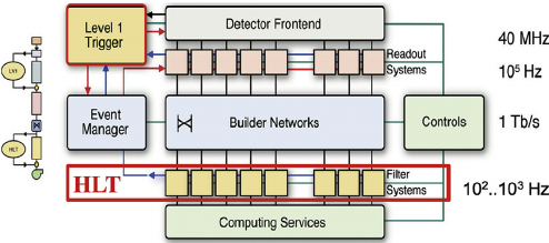
Collisions at the LHC happen at a rate close to 40 million per second (40 MHz). Once each collision is sensed by the different subdetectors, the amount of information they generate corresponds to about what you can fit in a 1 MB file. If we were to record every single collision, it is said (you can do the math) that one can probably fill out all the available disk space in the world in a few days!
Not all collisions that happen at the LHC are interesting. We would like to keep the interesting ones and, most importantly, do not miss the discovery-quality ones. In order to achieve that we need a Trigger.
Before we jump into the details for the trigger system, let’s agree on some terminology:
Fill: Every time the LHC injects beams in the machine it marks the beginning of what is known as a Fill.
Run: As collisions happen in the LHC, CMS (and the other detectors) decide whether they start recording data. Every time the start button is pushed, a new Run starts and it is given a unique number.
Lumi section: while colliding, the LHC’s delivered instantaneous luminosity gets degraded (although during Run 3 it will be mainly levelled) due to different reasons. I.e., it is not constant over time. For practical reasons, CMS groups the events it collects in luminosity sections, where the luminosity values can be considered constant.
The trigger system
Deciding on which events to record is the main purpose of the trigger system. It is like determining which events to record by taking a quick picture of it and, even though a bit blurry, decide whether it is interesting to keep or not for a future, more thorough inspection.
CMS does this in two main steps. The first one, the Level 1 trigger (L1), implemented in hardware (fast FPGAs), reduces the input rate of 40 Mhz to around 100 KHz. The other step is the High Level Trigger (HLT), run on commercial machines with good-old C++ and Python, where the input rate is leveled around the maximum available budget of around 2 KHz.
There are hundreds of different triggers in CMS. Each one of them is designed to pick certain types of events, with different intensities and topologies. For instance the HLT_Mu20 trigger, will select events with at least one muon with 20 GeV of transverse momentum.
At the HLT level, which takes L1 as input, triggers are implemented using the primary CMS software, CMSSW, using pieces of it (“modules”) that can be arranged to achieve the desired result: selecting specific kinds of events. Computationally, triggers are CMSSW “Paths”, and one could extract a lot of information by exploring the Python configuration of these paths. Within CMS, data is processed using C++ source code configured using Python. An example of a trigger path in a python configuration file might look like this:
PYTHON
process.HLT_Mu20_v2 = cms.Path( process.HLTBeginSequence + process.hltL1sL1SingleMu16 + process.hltPreMu20 + process.hltL1fL1sMu16L1Filtered0 + process.HLTL2muonrecoSequence + process.hltL2fL1sMu16L1f0L2Filtered10Q + process.HLTL3muonrecoSequence + process.hltL3fL1sMu16L1f0L2f10QL3Filtered20Q + process.HLTEndSequence )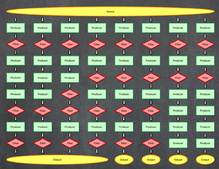
Triggers are code, and those pieces of code are constantly changing.
Modifications to a trigger could imply a different version identifier.
For instance, our HLT_Mu20 could actually be
HLT_Mu15_v1 or HLT_Mu15_v2, etc., depending on
the version. Therefore, it is completely normal that the trigger names
can change from run to run.
Prescales
The need for prescales (and its meaning) is evident if one thinks of
different physics processes having different cross sections. It is a lot
more likely to record one minimum bias event, than an event where a Z
boson is produced. Even less likely is to record an event with a Higgs
boson. We could have triggers named, say,
HLT_ZBosonRecorder for the one in charge of filtering
Z-carrying events, or HLT_HiggsBosonRecorder for the one
accepting Higgses (the actual names are more sophisticated and complex
than that, of course.) The prescales are designed to keep these
inputs under control by, for instance, recording just 1 out of 100
collisions that produce a likely Z boson, or 1 out of 1 collisions that
produce a potential Higgs boson. In the former case, the prescale would
be 100, while for the latter it would be 1; if a trigger has a prescale
of 1, i.e., records every single event it identifies, we call it
unprescaled.
Maybe not so evident is the need for trigger prescale changes for keeping up with luminosity changes. As the luminosity drops, prescales can be relaxed, and therefore could change from to run in the same fill. A trigger can be prescaled at L1 as well as the HLT levels. L1 triggers have their own nomenclature and can be used as HLT trigger seeds.
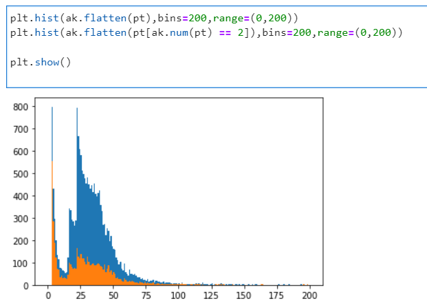
You saw the effect of trigger prescaling in the pre-exercise for dataset scouting. When plotting the muon momentum, several peaks and valleys appear at the low momentum edge. If the lower-momentum triggers were unprescaled, there would be many more events in the dataset with low pt muons, making a smoothly falling curve.
Triggers, streams and datasets
After events are accepted by possibly more than one type of trigger, they are streamed in different categories, called streams and then classified and arranged in primary datasets. Most, but not all, of the datasets belonging to the stream A, the physics stream, are or will become available as CMS Open Data.
Finally, it is worth mentioning that:
- an event can be triggered by many trigger paths
- trigger paths are unique to each dataset
- the same event can arrive in two different datasets (this is speciall important if working with many datasets as event duplication can happen and one has to account for it)
Key Points
- The CMS trigger system filters uninteresting events, keeping the budget high for the flow of interesting data.
- Computationally, a trigger is a CMSSW path, which is composed of several software modules.
- Trigger prescales allow the data acquisition to adjust to changes in instantaneous luminosity while keeping the rate of incomming data under control
- The trigger systems allows for the classification and organization of datasets by physics objects of interest.
Content from Triggers in NanoAOD
Last updated on 2024-07-18 | Edit this page
Estimated time: 15 minutes
Overview
Questions
- What information for triggers can I find in NanoAOD?
- What information is not available in NanoAOD?
Objectives
- Identify the L1 and HLT information in NanoAOD
- Learn alternate methods of accessing prescale information
- Access resources to learn about trigger object information in MiniAOD files
Triggers in NanoAOD
For many physics analyses, one basic piece of trigger information is required: did this event pass or fail a certain path? NanoAOD stores this information for both L1 and HLT paths. Let’s consider 3 example HLT paths:
- HLT_Ele35_WPTight_Gsf
- HLT_IsoMu27
- HLT_IsoMu27_LooseChargedIsoPFTauHPS20_Trk1_eta2p1_SingleL1
The first element of the name indicates that these paths are part of the “High Level Trigger” mentioned in the introduction. The second element of the name shows the first physics object that was tested for this path – the first example is an electron trigger, and the other two are muon triggers. Following the short name “Ele” or “Mu” is a momentum/energy threshold for this object, measured in GeV. The example “HLT_IsoMu27” has another feature in the name: “Iso”. This indicates that the muon is required to be isolated. Adding isolation requirements helps keep the momentum threshold for this popular trigger low without overwhelming the CMS trigger bandwidth.
The final example shows a trigger with multiple objects – after the “IsoMu27” label comes a label related to tau leptons: “LooseChargedIsoPFTauHPS20_Trk1_eta2p1_SingleL1”. This is a complex label that would share with experts many details of how the tau passing this trigger appeared in the CMS calorimeters. The most important information is that this tau lepton decayed to hadrons (note the “HPS” label for “hadron plus strips), was loosely isolated from other charged hadrons, passed a 20 GeV threshold, and was found in the central region of the detector (\(\eta < 2.1\)). This trigger might be used for a \(H \rightarrow \tau \tau\) analysis with one hadronic tau and one tau that decayed to a muon.
NanoAOD branch listings
Each dataset’s record page contains a link to its variable listing, which will show the full list of L1 and HLT paths available in that dataset. We will show short examples below.
Note:
- No version number appears in the branch names! NanoAOD assumes you want all versions of a trigger
- All the branches are type “bool”, so they indicate pass (true) or fail (false) for the event
- Some L1 paths relate to detector conditions, and some to energy thresholds
- Many triggers of the same type exist with a variety of energy or momentum thresholds
| Object property | Type | Description |
|---|---|---|
| L1_AlwaysTrue | Bool_t | Trigger/flag bit (process: NANO) |
| L1_BPTX_AND_Ref4_VME | Bool_t | Trigger/flag bit (process: NANO) |
| L1_BPTX_BeamGas_B1_VME | Bool_t | Trigger/flag bit (process: NANO) |
| L1_BPTX_BeamGas_B2_VME | Bool_t | Trigger/flag bit (process: NANO) |
| L1_BPTX_BeamGas_Ref1_VME | Bool_t | Trigger/flag bit (process: NANO) |
| L1_BPTX_BeamGas_Ref2_VME | Bool_t | Trigger/flag bit (process: NANO) |
| L1_BPTX_NotOR_VME | Bool_t | Trigger/flag bit (process: NANO) |
| L1_BptxMinus | Bool_t | Trigger/flag bit (process: NANO) |
| L1_BptxOR | Bool_t | Trigger/flag bit (process: NANO) |
| L1_BptxPlus | Bool_t | Trigger/flag bit (process: NANO) |
| L1_BptxXOR | Bool_t | Trigger/flag bit (process: NANO) |
| L1_CDC_SingleMu_3_er1p2_TOP120_DPHI2p618_3p142 | Bool_t | Trigger/flag bit (process: NANO) |
| L1_DoubleEG8er2p5_HTT260er | Bool_t | Trigger/flag bit (process: NANO) |
| L1_DoubleEG8er2p5_HTT320er | Bool_t | Trigger/flag bit (process: NANO) |
| L1_DoubleEG8er2p5_HTT340er | Bool_t | Trigger/flag bit (process: NANO) |
| L1_DoubleEG_15_10_er2p5 | Bool_t | Trigger/flag bit (process: NANO) |
| L1_DoubleEG_20_10_er2p5 | Bool_t | Trigger/flag bit (process: NANO) |
| Object property | Type | Description |
|---|---|---|
| HLT_Ele30_WPTight_Gsf | Bool_t | Trigger/flag bit (process: HLT) |
| HLT_Ele30_eta2p1_WPTight_Gsf_CentralPFJet35_EleCleaned | Bool_t | Trigger/flag bit (process: HLT) |
| HLT_Ele32_WPTight_Gsf | Bool_t | Trigger/flag bit (process: HLT) |
| HLT_Ele32_WPTight_Gsf_L1DoubleEG | Bool_t | Trigger/flag bit (process: HLT) |
| HLT_Ele35_WPTight_Gsf | Bool_t | Trigger/flag bit (process: HLT) |
| HLT_Ele35_WPTight_Gsf_L1EGMT | Bool_t | Trigger/flag bit (process: HLT) |
| HLT_Ele38_WPTight_Gsf | Bool_t | Trigger/flag bit (process: HLT) |
| HLT_IsoMu27 | Bool_t | Trigger/flag bit (process: HLT) |
| HLT_IsoMu27_LooseChargedIsoPFTauHPS20_Trk1_eta2p1_SingleL1 | Bool_t | Trigger/flag bit (process: HLT) |
| HLT_IsoMu27_MET90 | Bool_t | Trigger/flag bit (process: HLT) |
| HLT_IsoMu27_MediumChargedIsoPFTauHPS20_Trk1_eta2p1_SingleL1 | Bool_t | Trigger/flag bit (process: HLT) |
| HLT_IsoMu27_TightChargedIsoPFTauHPS20_Trk1_eta2p1_SingleL1 | Bool_t | Trigger/flag bit (process: HLT) |
| HLT_IsoMu30 | Bool_t | Trigger/flag bit (process: HLT) |
| HLT_IsoTrackHB | Bool_t | Trigger/flag bit (process: HLT) |
| HLT_IsoTrackHE | Bool_t | Trigger/flag bit (process: HLT) |
| HLT_Mu48NoFiltersNoVtx_Photon48_CaloIdL | Bool_t | Trigger/flag bit (process: HLT) |
| HLT_Mu4_TrkIsoVVL_DiPFJet90_40_DEta3p5_MJJ750_HTT300_PFMETNoMu60 | Bool_t | Trigger/flag bit (process: HLT) |
| HLT_Mu50 | Bool_t | Trigger/flag bit (process: HLT) |
| HLT_Mu50_IsoVVVL_PFHT450 | Bool_t | Trigger/flag bit (process: HLT) |
What is the “process”?
CMS processes data in many steps (RECO, HLT, PAT, NANO…). These branches in NanoAOD are marking for the user which processing step produced the information seen in the NanoAOD file.
L1 PreFiring corrections
The 2016 NanoAOD files also contain a set of branches labeled “L1PreFiringWeight”. In 2016 and 2017, the gradual timing shift of the ECAL was not properly propagated to the L1 trigger system, resulting in a significant fraction of high-\(\eta\) “trigger primitives” being mistakenly associated to the previous bunch crossing. Since Level-1 rules forbid two consecutive bunch crossings from firing, an unpleasant consequence of this is that events can effectively “self veto” if a significant amount of ECAL energy is found in the region \(2.0 < |\eta| < 3.0\). The effect is strongly \(\eta\)- and \(p_{T}\)-dependent and prefiring rates can be large for high-momentum jets in the forward regions of the detector. A similar effect is present in the muon system, where the bunch crossing assignment of the muon candidates can be wrong due to the limited time resolution of the muon detectors. This effect was most pronounced in 2016, and the magnitude varies between 0% and 3%.
The L1PreFiring table in NanoAOD provides weights that analysts can apply to simulation to correct for these effects, so that simulation better represents data. The weights carry associated uncertainties, represented in alternate branches.
| Object property | Type | Description |
|---|---|---|
| L1PreFiringWeight_Dn | Float_t | L1 pre-firing event correction weight (1-probability), down var. |
| L1PreFiringWeight_ECAL_Dn | Float_t | ECAL L1 pre-firing event correction weight (1-probability), down var. |
| L1PreFiringWeight_ECAL_Nom | Float_t | ECAL L1 pre-firing event correction weight (1-probability) |
| L1PreFiringWeight_ECAL_Up | Float_t | ECAL L1 pre-firing event correction weight (1-probability), up var. |
| L1PreFiringWeight_Muon_Nom | Float_t | Muon L1 pre-firing event correction weight (1-probability) |
| L1PreFiringWeight_Muon_StatDn | Float_t | Muon L1 pre-firing event correction weight (1-probability), down var. stat. |
| L1PreFiringWeight_Muon_StatUp | Float_t | Muon L1 pre-firing event correction weight (1-probability), up var. stat. |
| L1PreFiringWeight_Muon_SystDn | Float_t | Muon L1 pre-firing event correction weight (1-probability), down var. syst. |
| L1PreFiringWeight_Muon_SystUp | Float_t | Muon L1 pre-firing event correction weight (1-probability), up var. syst. |
| L1PreFiringWeight_Nom | Float_t | L1 pre-firing event correction weight (1-probability) |
| L1PreFiringWeight_Up | Float_t | L1 pre-firing event correction weight (1-probability), up var. |
What’s missing from NanoAOD?
NanoAOD does not contain information about trigger prescales or objects:
- The prescale is a “scale down factor” for triggers with rates too high to record all events
- A trigger object is a link to the electron, muon, jet, tau, etc, that specifically satisfied the criteria for a given trigger filter
Prescale information is fixed in the “trigger menu”, so it can be
accessed outside of NanoAOD. While it’s common for prescale values to
change from run to run, most analysts are only interested in determining
whether or not a trigger is prescaled at all. If not, that trigger is a
good candidate for analyses requiring the full amount of data available.
If so, the trigger is better suited to studies where statistics are not
a limiting factor. Prescale values for any trigger can be accessed from
the brilcalc tool that we will discuss in the upcoming
episodes. We will practice finding a prescale value as an exercise.
Trigger object information is important if an analysis needs to know
which specific objects passed a certain set of trigger filters. So for
instance, if you needed to know which tau leptons satisfied
LooseChargedIsoPFTauHPS20_Trk1_eta2p1_SingleL1 in order to
make correct analysis choices, then you would need access to trigger
object details. Many analyses do not require this level of detail, since
physics objects can usually be selected using the identification and
isolation algorithms designed to be applied separately from the trigger
system. Trigger objects can be accessed in MiniAOD – follow our trigger
lesson for 2015 MiniAOD from 2023 to learn more.
Key Points
- NanoAOD stores basic pass/fail information for both L1 and HLT paths
- NanoAOD does not contain trigger prescale or trigger object information
- Trigger prescale information can be accessed from brilcalc
- Trigger object information must be accessed by processing MiniAOD files in CMSSW
Content from Luminosity
Last updated on 2024-07-18 | Edit this page
Estimated time: 15 minutes
Overview
Questions
- What does “luminosity” mean in particle physics?
- How is luminosity measured in CMS?
- How is integrated luminosity calculated?
Objectives
- Understand the significance of luminosity to collider physics.
- Learn about the CMS luminometers.
- Learn the basic principles of computing luminosity values.
2016 luminosity paper
The information in this section is all from the 2015-2016 luminosity paper by CMS!
In collider physics, discovery potential can be summarized with two pieces of information:
- center-of-mass collision energy, \(\sqrt{s}\), that drives the range of produced particle masses, and
- luminosity, \(\mathcal{L}\), that drives the size of the accumulated dataset.
Luminosity can be measured for small moments in time (instantaneous luminosity) or integrated over a full data-taking period (integrated luminosity). CMS and the LHC use instantaneous luminosity information to understand the collision environment during data-taking. The integrated luminosity value is used by all analysts to measure cross sections of a process being studied, or to determine the number of events expected for physics processes with well-known cross sections. Luminosity is the ratio of the production rate, \(R\), (or number of produced events, \(N\)) and the “cross section” for the considered process:
\(\mathcal{L}(t) = R(t)/\sigma,\)
\(\mathcal{L}_{\mathrm{int.}} = N/\sigma.\)
Cross section is measured in “barns”, a unit of area relevant for nuclear-scale processes. The most literal meaning of the word cross section would describe cutting a (spherical?) atomic nucleus in half through the middle, exposing a circular flat surface. As targets for projectiles in nuclear reactions, most atomic nuclei “look” fairly circular, and the circles would have areas on the order of 10-100 square femtometers. A “barn” is exactly 100 square femtometers, or \(1 \times 10^{-28}\) square meters. Luminosity is therefore measured in the even stranger unit of inverse barns!
Typical cross sections for particle physics interactions are much smaller than nuclear physics interactions, ranging from millibarns down to femtobarns. The integrated luminosities required to discover these interactions grows as the cross section shrinks.
CMS Luminometers
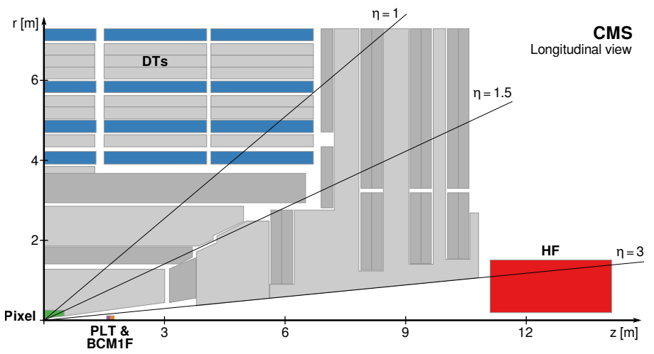
CMS has several subdetectors that serve as “luminometers”:
- Pixels: pixel tracking detector, which covers \(|\eta| < 2.5\)
- HF: forward hadron calorimeter, which covers \(3 < |\eta| < 5.2\)
- PLT: pixel luminosity telescope, an array of 16 “telescopes” with pixel sensors in planes facing the interaction point.
- BCM1F: the fast beam conditions monitor, a system of diamond sensors on the PLT apparatus.
The pixel detector contributes two measurements that are used for luminosity calculations: the number of charge clusters observed, and the number of vertices found with more than 10 tracks. The number of clusters can be used to compute the cross section for producing “visible particles”. It is vanishingly unlikely that particles overlap each other in the pixel detector, so the average number of clusters in the pixel detector tracks directly with the number of simultaneous collisions in CMS. The visible cross section is the slope, or ratio, of this relationship.
In the HF, a suite of FPGA readout electronics processes data at the full 40 MHz LHC collision rate. The record the number of channels in which above-threshold charge was deposited during the bunch crossing. The PLT looks for tracks from the collision point that hit all three sensors in one of the telescopes – the fraction of events with no PLT coincidences can be used in the luminosity calculation. The BCM1F has readout that is optimized for time precision. This subdetector has a time resolution of just over 6 ns, so it can separate collision hits from beam-related background hits. The data from all of these luminometers can be used to converge on a precise, stable determination of the luminosity in CMS.
Luminosity calculation and calibration
The true mean number of interations per LHC bunch crossing, \(\mu\), is proportional to the instantaneous luminosity of the bunch crossing:
\(\mu = \sigma \mathcal{L}_b / v_r\),
where \(v_r = 11 245.6\) Hz is the revolution frequency of the LHC, and \(\sigma\) is the total interaction cross section.
In the pixel detector, \(\mathcal{L}_b\) can be estimated from this formula by considering the average number of clusters and the visible cross section obtained by comparing the number of clusters to number of interactions. This algorithm is known as “rate scaling”:
\(\mathcal{L}_b = N_{\mathrm{av}} v_r / \sigma_{\mathrm{vis}}.\)
For the HF, PLT, and BCM1F luminometers, the “zero counting” method gives a better luminosity estimate, since these detectors are more likely than the pixel detectors to have multiple signals overlap and be counted as one observation. The number of interactions per bunch crossing is governed by the Poisson distribution, so if there is a probability \(p\) for an interaction result in 0 observations in a luminometer and \(k\) interactions in a given bunch crossing, the expected fraction of “empty” events, \(\langle f_0 \rangle\), can be written as the sum of the Poisson distribution times the total probability for all possible values of \(k\):
\(\langle f_0 \rangle = \sum_{k = 0}^{\infty}{\frac{e^{-\mu} \mu^k}{k!} p^k} = e^{-\mu(1-p)}\).
The true mean number of interactions per bunch cross can be extracted from this formula and related to the instantaneous luminosity per bunch crossing:
\(\mathcal{L}_b = \frac{-\ln\langle f_0 \rangle}{1-p} \frac{v_r}{\sigma}.\)
We can measure the visible cross section, \(\sigma_{\mathrm{vis}}\), from the pixel detector, which is effectively \((1-p)\sigma\), since \(1-p\) is the probability for an interaction to produce hits in a luminometer. The luminosity from the zero-counting method is then:
\(\mathcal{L}_b = -\ln\langle f_0 \rangle v_r/\sigma_{\mathrm{vis}}\).
The two methods produce very similar formulas based on different observables. After computing the per-bunch-crossing luminosity with these methods, a wide array of calibration methods are employed to ensure the precision and accuracy of the result. Beam-separation scans, information from independent detectors such as the muon drift tubes, beam position and current monitoring data, and more are used to compute corrections and uncertainties in the luminosity measurement.
For 2016, the total integrated luminosity is 36.3 fb\(^{-1}\), with an uncertainty of 1.2%. The paper notes that, “The final precision is among the best achieved at bunched-beam hadron colliders” – a great achievement!
Key Points
- Luminosity is a measure of the number of collisions occuring in CMS.
- Luminosity is measured in various subdetectors: the pixel tracker, the HF, the PLT, and the BCM1F.
- After careful calibration, the 2016 luminosity uncertainty is only 1.2%.
Content from Trigger & Lumi challenge
Last updated on 2024-07-18 | Edit this page
Estimated time: 30 minutes
Overview
Questions
- Which triggers are likely the most useful for selecting top quark events?
- What are the prescale values of some possible triggers?
- What is the luminosity collected by my chosen trigger?
Objectives
- Learn to make trigger choices based on analysis goals, expected physics objects, and available trigger paths.
- Practice using brilcalc to extract trigger prescale information
- Practice using brilcalc to compute integrated luminosity
Workshop analysis example: \(Z' \rightarrow t\bar{t} \rightarrow (bjj)(b\ell\nu)\)
Later in the workshop we will search for a Z’ boson that decays to a top quark-antiquark pair. The signal for this measurement is one top quark that decays hadronically, and one top quark that decays leptonically, to either a muon or an electron. For Z’ bosons with mass in the 1 - 5 TeV range, the top quarks should both be produced with high momentum.
Choosing a trigger path
Using what you have learned about CMS physics objects and triggers, let’s sketch out some ideas for potential trigger selections. To begin with:
Which final state particles would you expect to observe in the detector from your “signal” process?
Based on these particles, consider:
- Which physics objects could appear in a useful trigger path? At a hadron collider, which physics objects might be best for triggering?
- What kinematic conditions do you expect for the trigger physics objects?
- We saw trigger “trade-offs”, like requiring isolated particles in exchange for lower momenta – would that trade-off be beneficial in this case?
Physics exercise: choose trigger paths
Visit the NanoAOD HLT branch listing for our signal sample and choose 3-4 trigger options that might be effective for selecting \(Z' \rightarrow t\bar{t}\) events
For the \(t\bar{t}\) final state we will consider, we expect one electron or muon, MET from the accompanying neutrino, and several jets, some of which could be tagged as b quark jets. There might even be “fat jets” tagged as entire top quark decays. This analysis is perfect for the common “single lepton” triggers. Since the top quarks will be produced with high momentum, the lepton might not be well separated from a b quark jet, so it would be wisest to include a non-isolated trigger. Since the signal will likely produce high-pT leptons, we can afford to use triggers that require higher momentum in order to relax isolation requirements.
The triggers used in the CMS analysis that we are mimicking were:
- HLT_Mu50
- HLT_Ele50_CaloIdVT_GsfTrkIdT_PFJet165
- HLT_Ele115_CaloIdVT_GsfTrkIdT
For any of these triggers, the leptons (and jet, if applicable) should ideally be selected using criteria that put them in the “efficiency plateau” of the trigger. For example, the HLT_Mu50 trigger is designed to select muons with at least 50 GeV of transverse momentum, but if you plotted the number of muons selected as a function of pT, you would certainly not see a vertical line step function with 0 muons selected below 50 GeV and 100% of muons selected above 50 GeV. Right in the region of the threshold there will be a “turn-on” effect where the efficiency rises quickly, but not exactly following a step function. This turn-on can be difficult to model well in simulation, so many analysts choose selection criteria for physics objects that will not be subject to the turn-on effects of the trigger. For example, in an analysis using HLT_Mu50, the muon selection criteria would typically be pT > 55 GeV.
Brilcalc exercises
Exercise 1: test brilcalc
As a test, let’s see what the integrated luminosity was for run 284044 by running the command:
Note: It is important that you use the -c web option
when running brilcalc. This specifies that you use indirect access to
BRIL servers via a web cache. For users of CMS open data outside CERN
and CMS this is the only option that will work.
You should see the following output:
OUTPUT
#Data tag : 24v1 , Norm tag: onlineresult
+-------------+-------------------+-----+------+-------------------+-------------------+
| run:fill    | time              | nls | ncms | delivered(/ub)    | recorded(/ub)     |
+-------------+-------------------+-----+------+-------------------+-------------------+
| 284044:5451 | 10/26/16 20:46:05 | 594 | 40   | 5450634.956154574 | 4912825.742705812 |
+-------------+-------------------+-----+------+-------------------+-------------------+
#Summary:
+-------+------+-----+------+-------------------+-------------------+
| nfill | nrun | nls | ncms | totdelivered(/ub) | totrecorded(/ub)  |
+-------+------+-----+------+-------------------+-------------------+
| 1     | 1    | 594 | 40   | 5450634.956154574 | 4912825.742705812 |
+-------+------+-----+------+-------------------+-------------------+
Exercise 2: 2016 validated runs & luminosity sections
All CMS data is studied by data quality monitoring groups for various
subdetectors to determine whether it is suitable for physics analysis.
Data can be accepted or rejected in units of “luminosity sections”.
These are periods of time covering \(2^{18}\) LHC revolutions, or about 23
seconds. The list of validated runs and luminosity sections is stored in
a json file that can be downloaded from the Open Data
Portal.
First, obtain the file with the list of validated runs and luminosity sections for 2016 data:
BASH
wget https://opendata.cern.ch/record/14220/files/Cert_271036-284044_13TeV_Legacy2016_Collisions16_JSON.txtUse brilcalc to display the luminosity for each valid
run in the 2016 Open Data. Currently, we have released 2016G and 2016H
data, which contain runs 278820 through 284044.
BASH
brilcalc lumi -c web -b "STABLE BEAMS" --begin 278820 --end 284044 -i Cert_271036-284044_13TeV_Legacy2016_Collisions16_JSON.txt > 2016GHlumi.txt- Can you identify the run in this range that had the most luminosity sections?
- What is the total recorded luminosity for this run range?
You can investigate the output file best using head:
The longest run is 279931!
OUTPUT
#Data tag : 24v1 , Norm tag: onlineresult
+-------------+-------------------+------+------+---------------------+---------------------+
| run:fill    | time              | nls  | ncms | delivered(/ub)      | recorded(/ub)       |
+-------------+-------------------+------+------+---------------------+---------------------+
| 278820:5199 | 08/14/16 11:00:52 | 1524 | 1524 | 300457014.643834889 | 287580217.903829336 |
| 278822:5199 | 08/14/16 21:52:48 | 1627 | 1627 | 195829703.718308955 | 189724216.323258847 |
| 278873:5205 | 08/15/16 23:25:46 | 67   | 60   | 12468667.004980152  | 2012170.733444575   |
| 278874:5205 | 08/15/16 23:51:54 | 484  | 484  | 88533994.547763854  | 82142606.203014016  |
| 278875:5205 | 08/16/16 03:01:21 | 834  | 834  | 120598272.705723718 | 115092509.056569114 |
| 278923:5206 | 08/16/16 12:16:33 | 413  | 413  | 103255455.458636224 | 98881486.964829206  |
...
| 279887:5270 | 09/01/16 23:20:53 | 319  | 319  | 76790312.907530844  | 72932440.002667427  |
| 279931:5274 | 09/02/16 11:37:40 | 2936 | 2936 | 485408960.517024338 | 470459175.415192366 |
| 279966:5275 | 09/03/16 09:20:25 | 363  | 363  | 95862775.891636893  | 91937407.130460218  |
| 279975:5276 | 09/03/16 14:45:09 | 1024 | 1024 | 244951346.260912448 | 235979324.421879977 |
The units are inverse microbarns as default and can be changed to
inverse femtobarns with the option -u /fb.
The total recorded luminosity for the run range is listed in the summary below the individual runs:
OUTPUT
#Summary:
+-------+------+-------+-------+-----------------------+-----------------------+
| nfill | nrun | nls   | ncms  | totdelivered(/ub)     | totrecorded(/ub)      |
+-------+------+-------+-------+-----------------------+-----------------------+
| 64    | 156  | 90807 | 90526 | 17062540322.934297562 | 16290713419.734096527 |
+-------+------+-------+-------+-----------------------+-----------------------+
CMS recorded 16.3 inverse femtobarns of proton-proton collisions in 2016 G and H!
Exercise 3: selecting the best luminometer
Update to
For Run-2 data, the luminometer giving the best value for each luminosity section is recorded in a ‘normtag’ file, provided in the 2016 luminosity information record (‘normtag_PHYSICS_pp_2016.json’). Use it with the corresponding list of validated runs from 2016 to find the best estimate of the 2016G-H luminosity.
BASH
wget https://opendata.cern.ch/record/1059/files/normtag_PHYSICS_pp_2016.json
brilcalc lumi -c web -b "STABLE BEAMS" --begin 278820 --end 284044 -i Cert_271036-284044_13TeV_Legacy2016_Collisions16_JSON.txt -u /fb --normtag normtag_PHYSICS_pp_2016.json > 2016GHlumi_normtag.txt
Does it change compared to the previous exercise?
The summary should now read:
OUTPUT
#Summary:
+-------+------+-------+-------+-------------------+------------------+
| nfill | nrun | nls   | ncms  | totdelivered(/fb) | totrecorded(/fb) |
+-------+------+-------+-------+-------------------+------------------+
| 64    | 156  | 90807 | 90526 | 17.168970230      | 16.393380532     |
+-------+------+-------+-------+-------------------+------------------+
To three significant figures, the luminosity is better reported as 16.4 inverse femtobarns.
Exercise 4: Luminosity and prescale values for an HLT trigger path
One of the triggers that is a good candidate for the Z’ search
example is HLT_Mu50. Let’s calculate the integrated
luminosity covered by this trigger for the long run 279931:
Compare this luminosity to the similar trigger HLT_Mu27
– what difference do you observe? What is happening to Mu27 that is not
occurring for Mu50?
In run 279931, the luminosity collected with Mu50* is:
OUTPUT
+-------------+-------------------+------+-----------------------------+---------------------+---------------------+
| run:fill    | time              | ncms | hltpath                     | delivered(/ub)      | recorded(/ub)       |
+-------------+-------------------+------+-----------------------------+---------------------+---------------------+
| 279931:5274 | 09/02/16 11:36:53 | 2945 | HLT_Mu50_IsoVVVL_PFHT400_v3 | 486636050.343178093 | 471451252.657074332 |
| 279931:5274 | 09/02/16 11:36:53 | 2945 | HLT_Mu50_v4                 | 486636050.343178093 | 471451252.657074332 |
+-------------+-------------------+------+-----------------------------+---------------------+---------------------+
The luminosity collected with Mu27* is:
OUTPUT
+-------------+-------------------+------+--------------------------------------+---------------------+---------------------+
| run:fill    | time              | ncms | hltpath                              | delivered(/ub)      | recorded(/ub)       |
+-------------+-------------------+------+--------------------------------------+---------------------+---------------------+
| 279931:5274 | 09/02/16 11:36:53 | 2945 | HLT_Mu27_Ele37_CaloIdL_GsfTrkIdVL_v4 | 486636050.343178093 | 471451252.657074332 |
| 279931:5274 | 09/02/16 11:36:53 | 2945 | HLT_Mu27_TkMu8_v3                    | 334796076.249607444 | 325826000.870547831 |
| 279931:5274 | 09/02/16 11:36:53 | 2945 | HLT_Mu27_v4                          | 3373601.765050163   | 3273957.230715709   |
+-------------+-------------------+------+--------------------------------------+---------------------+---------------------+
The Mu27 trigger is significantly prescaled!
Note: you could combine the example in this exercise with the
brilcalc options --begin, --end,
-i, and --normtag to confirm the total
integrated luminosity for a given trigger path. This command can take a
while! If you wish to use wildcards to get results for many trigger
paths, you can consider adding --output-style csv and
redirecting the results to a .csv file for easier analysis.
OUTPUT
+--------+-------+----------+-------------+--------------------+-------+---------------------------------------+
| run    | cmsls | prescidx | totprescval | hltpath/prescval   | logic | l1bit/prescval                        |
+--------+-------+----------+-------------+--------------------+-------+---------------------------------------+
| 279931 | 1     | 2        | 260.00      | HLT_Mu27_v4/260    | OR    | L1_SingleMu22/1.00 L1_SingleMu25/1.00 |
| 279931 | 71    | 6        | 140.00      | HLT_Mu27_v4/140    | OR    | L1_SingleMu22/1.00 L1_SingleMu25/1.00 |
| 279931 | 74    | 2        | 260.00      | HLT_Mu27_v4/260    | OR    | L1_SingleMu22/1.00 L1_SingleMu25/1.00 |
| 279931 | 262   | 3        | 230.00      | HLT_Mu27_v4/230    | OR    | L1_SingleMu22/1.00 L1_SingleMu25/1.00 |
| 279931 | 521   | 4        | 200.00      | HLT_Mu27_v4/200    | OR    | L1_SingleMu22/1.00 L1_SingleMu25/1.00 |
| 279931 | 752   | 5        | 160.00      | HLT_Mu27_v4/160    | OR    | L1_SingleMu22/1.00 L1_SingleMu25/1.00 |
| 279931 | 1088  | 6        | 140.00      | HLT_Mu27_v4/140    | OR    | L1_SingleMu22/1.00 L1_SingleMu25/1.00 |
| 279931 | 1946  | 7        | 100.00      | HLT_Mu27_v4/100    | OR    | L1_SingleMu22/1.00 L1_SingleMu25/1.00 |
The total prescale value is the product of any prescale applied at L1
with any prescale applied at HLT. As this long run proceeded, the
prescale values changed several times. During a portion of the run this
trigger was not allowed to collect any luminosity, and in other portions
it was scaled down by at least a factor of 100. In contrast, you can
confirm that Mu50 always has a prescale of 1. Any wildcard can be given
in the --hltpath option to compare many triggers for a
certain physics object and find unprescaled options.
Key Points
- Triggers need to be chosen with the event topology of the analysis in mind! They place constraints on your choices for selecting physics objects in an analysis.
- The brilcalc tools allows you to calculate luminosity for a run, a range of runs, or a trigger path.
- The brilcalc tool can also share information about trigger prescales throughout a run.