Limit calculation challenge
Last updated on 2024-08-01 | Edit this page
Estimated time: 40 minutes
Overview
Questions
- How do I write a Combine datacard for a counting analysis and for a shape analysis?
- How do I incorporate the effects of systematic uncertainties?
- How do I calculate expected and observed limits?
- How do I interpret the resulting limits?
Objectives
- Construct a Combine datacard for a counting analysis, learn to modify systematics.
- Construct a Combine datacard for a shape analysis, learn to modify systematics.
- Calculate limits using Combine with different methods for counting and shape datacards and compare.
- Understand what the limits mean.
The goal of this exercise is to use the Combine tool to
calculate limits from the results of the \(Z'\) search studied in the previous
exercises. We will use the Zprime_hists_FULL.root file
generated during the Uncertainties
challenge. We will build various datacards from it, add systematics,
calculate limits on the signal strength modifier and understand the
output.
Prerequisite
For the activities in this session you will need:
- Your Combine docker container (installation instructions provided in the setup section of this tutorial)
Statistical analysis as a counting experiment
At the end of the https://cms-opendata-workshop.github.io/workshop2024-lesson-event-selection/,
you applied a set of selection criteria to events that would enhance
\(Z'\) signal from SM backgrounds.
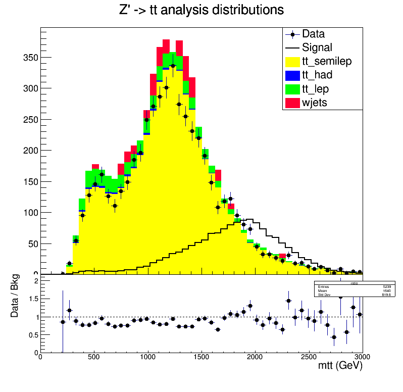
Then you obtained the ttbar mass distributions for data, \(Z'\) signal and a set of SM background
processes after this selection. In the Uncertainties
challenge exercise, you learned to obtain variations on these
distributions arising from certain systematic effects. In this first
exercise, we will treat the events surviving the selection as a single
quantity to perform a statistical analysis on a counting experiment. In
other words, we will collapse the mtt distributions into a
single “number of events” by integrating over all bins. Then we will use
these numbers obtained for all histograms, including those with
systematic variations, to build a counting experiment datacard.
First, start your Combine Docker container and make a working directory:
Download the Zprime_hists_FULL.root and the python
script to make the datacard:
BASH
wget https://github.com/cms-opendata-workshop/workshop2024-lesson-statistical-inference/raw/main/instructors//Zprime_hists_FULL.root
wget https://github.com/cms-opendata-workshop/workshop2024-lesson-statistical-inference/raw/main/instructors//writecountdatacard.py
You can look into the writecountdatacard.py script to
see how the datacard is written from the ROOT file. Run the script:
(ignore the output for the moment). Now look into
datacard_counts.txt and try to answer the following
questions:
Questions
- Which is the background contributing most?
- What can you say when you compare data, total backgrounds, and signal counts?
- Can you understand the effect of the various systematic uncertainties?
- Which systematic is expected to have the overall bigger impact?
- Which process is affected most by systematics?
Now run Combine over this datacard to obtain the limits on our
parameter of interest, signal strength modifier, with the simple
AsymptoticLimits option:
You will see some error messages concerning the computation of the observed limit, arising from numerical stability issues. In order to avoid this, let’s rerun by limiting the signal strength modifier to be maximum 2:
Look at the output, and try to answer the following:
Questions
- What is the observed limit? What is the expected limit? What are the uncertainties on the expected limit?
- Did our analysis exclude this particular \(Z'\) signal?
- What can you say when you compare the values of the observed limit with the expected limit?
- What does it mean that the observed limit is much lower compared to the expected limit? Does this make sense? Hint: Go back to the datacard and look at the data, background and signal counts.
Taming the observed (DON’T TRY THIS AT HOME!)
A hypothetical question: What would bring the observed limit within the expected uncertainties? Do the necessary modifications in the datacard and see if the limit behaves as you predicted.
You can rerun writecountdatacard.py to reset the
datacard.
Observed limit is below the expected boundaries because we have much more MC compared to data. This means there is less room for signal to be accommodated in data, i.e. excluding signal becomes easier. If we had more data, or less backgrounds, there would be more room for signal, and the observed limit would be more consistent with the expected. So hypothetically one could
- Increase the data counts, or
- Decrease counts in one or more background processes.
The point of this question was to increase the understanding. We never do this in real life!!!
Add uncertainties to the datacard
Now let’s add more uncertainties, both systematic and statistical. Let’s start with adding a classic - the systematic uncertainty due to luminosity measurement:
Challenge: Add a lognormal luminosity systematic
- Please add a lognormal systematic uncertainty on luminosity (called
lumi) that affects all signal and background processes, inducing a symmetric 2.5% up and down variation. - Run Combine with the new datacard and discuss the effect on the limits.
lumi lnN 1.025 1.025 1.025 1.025 1.025Now let’s add a statistical uncertainty. Our signal and background yields come from Monte Carlo, and the number of events could be limited, resulting on non-negligible statistical uncertainties. We apply event weights to these MC events so that the resulting rate matches a certain value, e.g. cross section times the luminosity. Statistical uncertainties are particularly relevant if both the yields are small and the event weights are large (i.e. much less actual MC events are available compared to the expected yield). Here is a quote from the Combine documentation on how to take these into account:
“gmN stands for Gamma, and is the recommended choice for the statistical uncertainty in a background determined from the number of events in a control region (or in an MC sample with limited sample size). If the control region or simulated sample contains N events, and the extrapolation factor from the control region to the signal region is α, one shoud put N just after the gmN keyword, and then the value of α in the relevant (bin,process) column. The yield specified in the rate line for this (bin,process) combination should equal Nα.”
Now let’s get back to the output we got from running
writecountdatacard.py. There you see the number of total
unweighted events, total weighted events and event weight for each
process.
Challenge: Add a statistical uncertainty
Look at the output of writecountdatacard.py:
- Which process has the largest event weight?
- Can you incorporate the statistical uncertainty for that particular process to the datacard?
- Run Combine and discuss the effect on the limits.
- OPTIONAL: You can add the statistical uncertainties for the other processes as well and observe their effect on the limits.
stat_signal     gmN 48238  0.0307         -              -              -              -
stat_tt_semilep gmN 137080 -              0.0383         -              -              -
stat_tt_had     gmN 817    -              -              0.0636         -              -
stat_tt_lep     gmN 16134  -              -              -              0.0325         -
stat_wjets	gmN 19     -              -              -              -              15.1623
Improve the limit
Improving the limit
What would you do to improve the limit here?
Hint: Look at the original plot displaying the data, background and signal distributions.
- In a count experiment setup, we can consider taking into account a
part of the
mttdistribution where the signal is dominant. - We can do a shape analysis, which takes into account each bin separately.
Let’s improve the limit in the couting experiment setup by computing total counts considering only the last 25 bins out of the 50 total:
We also added flags to automatically add the satistical and lumi uncertainties :). How did the yields change? Did the limit improve? You can try with different starting bin options to see how the limits change.
Shape analysis
Now we move to a shape analysis, where each bin in the
mtt distribution is taken into account. Datacards for shape
analyses are built with similar principles as those for counting
analyses, but their syntax is slightly different. Here is the shape
datacard for the \(Z'\)
analysis:
BASH
wget https://github.com/cms-opendata-workshop/workshop2024-lesson-statistical-inference/raw/main/instructors/datacard_shape.txtExamine it and note the differences in syntax. To run on Combine,
this datacard needs to be accompanied by the
Zprime_hists_FULL.root file, as the shapes are directly
retrieved from the histograms within.
Run Combine with this datacard. How do the limits compare with respect to the counts case?
Limits on cross section
So far we have worked with limits on the signal strength modifier. How can we compute the limits on cross section? Can you calculate the upper limit on \(Z'\) cross section for this model?
We can multiply the signal strength modifier limit with the theoretically predicted cross section for the signal process.