Introduction to statistical inference
Last updated on 2024-08-01 | Edit this page
Estimated time: 20 minutes
Overview
Questions
- What does statistical inference mean?
- What is a statistical model and a likelihood?
- What types of statistical models do we use?
- How do we incorporate constraints on nuisance parameters?
Objectives
- Understand the role of statistical inference in an analysis and related terminology.
- Understand the concept of a statistical model and a likelihood.
- Learn the types of statistical models generally used in analyses.
- Learn how the constraints on nuisance parameters are implemented.
Reference Material
- Combine Manual
- Combine Tutorial at LPC
- Practical Statistics for LHC Physicists - Three CERN Academic Lectures by Harrison Prosper
- Statistics in Theory - A lecture by Bob Cousins
- RooFit - Slides by Wouter Verkerke, one of the RooFit developers
- RooFit Tutorials - A set of macros that showcase all major features of RooFit
- RooStats Manual - A concise, clear, summary of statistics concepts and definitions
- RooStats Tutorial - Tutorial by Kyle Cranmer, one of the RooStats developers
- RooStats Tutorials - A set of macros that showcase all major features of RooStats
- CMS DAS 2014 Statistics Exercise - A tutorial on statistics as used in CMS
- Procedure for the LHC Higgs boson search combination in Summer 2011 - Paper describing LHC statistical procedures
- Combine Github - Github repository for combine
- LPC statistics course - Lectures by Harrison Prosper and Ulrich Heintz, fall 2017
Terminology and Conventions
Here we give pragmatic definitions for a few basic concepts that we will use.
- observable - something you measure in an experiment, for example, a particle’s momentum. Often, a function of measured quantities, for example, an invariant mass of several particles.
- global observable or auxiliary observable - an observable from another measurement, for example, the integrated luminosity.
- model - a set of probability functions (PFs) describing the distributions of observables or functions of observables. The probability functions are called probability density functions (PDFs) if the observables are continuous and probability mass functions (PMF) if the observables are discrete. In the Bayesian approach, the model also includes the prior density.
- model parameter - any variable in your model that is not an observable.
- parameter of interest (POI) - a model parameter of current interest, for example, a cross section.
- nuisance parameter - every model parameter other than your parameter (or parameters) of interest.
- data or data set - a set of values of observables, either measured in an experiment or simulated.
- likelihood - a model computed for a particular data set.
- hypothesis - a model in which all quantities are specified: observables, model parameters, and prior PDFs (in case of Bayesian inference).
- prior - a probability or probability density for an observable or a model parameter that is independent of the data set. Priors are a key feature of Bayesian inference. However, priors can be used in frequentist inference only if they can be interpreted as relative frequencies.
- Bayesian - a school of statistical inference based on the likelihood and a prior.
- frequentist - a school of statistical inference based on the likelihood only.
Statistical inference is the last step of an analysis and plays a crucial role in interpreting the experimental data. It involves using statistical methods to draw conclusions about the underlying physical processes based on observed data. This process includes defining a statistical model, constructing a likelihood function, and employing techniques such as hypothesis testing and parameter estimation to extract meaningful insights. Let’s start with the concept of a statistical model.
Statistical model
Statistical model is the mathematical framework used to describe and make inferences about the underlying processes that generate observed data. It encodes the probabilistic dependence of the observed quantities (i.e. data) on parameters of the model. These parameters are not directly observable but can be inferred from experimental data. They include
- parameters of interest (POI), \(\vec{\mu}\): The quantities we are interested in estimating or testing. Examples are cross section, signal strength modifier, resonance mass, …
- nuisance parameters, \(\vec{\nu}\): parameters that are not of direct interest, but required to explain data. These could be uncertainties of experimental or theoretical origin, such as detector effects, background measurements, lumi calibration, cross-section calculation.
Data are also partitioned into two:
- primary observables, \(\vec{x}\): Appear in components of the model that contain the POIs.
- auxiliary observables, \(\vec{y}\): Appear only in components of the model that contain the nuisance parameters.
Likelihood is the value of the statistical model at a given fixed set of data as a function of parameters.
Statistical model provides the complete mathematical description of an analysis and is the starting point of any interpretation.
Now let’s express this mathamatically. Our statistical model be described as \(p(\rm{data,\vec{\Phi}})\) where \(\vec{\Phi}\) are the model parameters. For the sake of numerical efficiency, we can factorize it into two parts:
\[p(\vec{x},\vec{y};\vec{\Phi}) = p(\vec{x};\vec{\mu},\vec{\nu}) \prod_k p_k(\vec{y}_k;\vec{\nu}_k)\]
- primary component: \(p(\vec{x};\vec{\mu},\vec{\nu})\). Relates POI to primary observables.
- auxiliary component: \(\prod_k p_k(\vec{y}_k;\vec{\nu}_k)\). Constrains nuisance parameters.
Likelihood function is constructed by evaluating \(p(\rm{data,\vec{\Phi}})\) on a dataset:
\[L(\vec{\Phi}) = \prod_d p(\vec{x}_d;\vec{\mu},\vec{\nu}) \prod_k p_k(\vec{y}_k;\vec{\nu}_k)\]
where \(d\) runs over all entries in data.
This likelihood can be used in both frequentist and Bayesian calculations.
Types of statistical models
Counting analysis
A counting analysis is one for which the statistical model has only one primary observable, namely the total event count in a single channel that includes multiple sources of signal and background. In the following, the primary observable is labeled \(n\). The probability to observe \(n\) events is described by a Poisson distribution,
\[p(n;\lambda(\vec{\mu}, \vec{\nu})) =\lambda^n\frac{e^{-\lambda}}{n!}\]
where the expected value, \(\lambda\), can be a function of one or more parameters, and represents the total number of expected signal and background events.
For our analyses, we usually express \(\lambda\), the expected number of events as:
\[\lambda \equiv n_{exp} = \mu \rm{\sigma_{sig}^{eff}} L + \rm{\sigma_{bg}^{eff}} L\]
Here \(\rm{\sigma_{sig}^{eff}}\) and \(\rm{\sigma_{bg}^{eff}}\) are signal and background effective cross sections (i.e. cross section times selection efficiency times detector acceptance) and \(L\) is the integrated luminosity. Our parameter of interest here is \(\mu\), the signal strength modifier. The estimated value of \(\mu\) would be able to tell us if the signal is discovered, excluded or still out of reach.
Template shape analysis
A shape analysis is defined as one that incorporates one or more primary observables, beyond a single number of events.
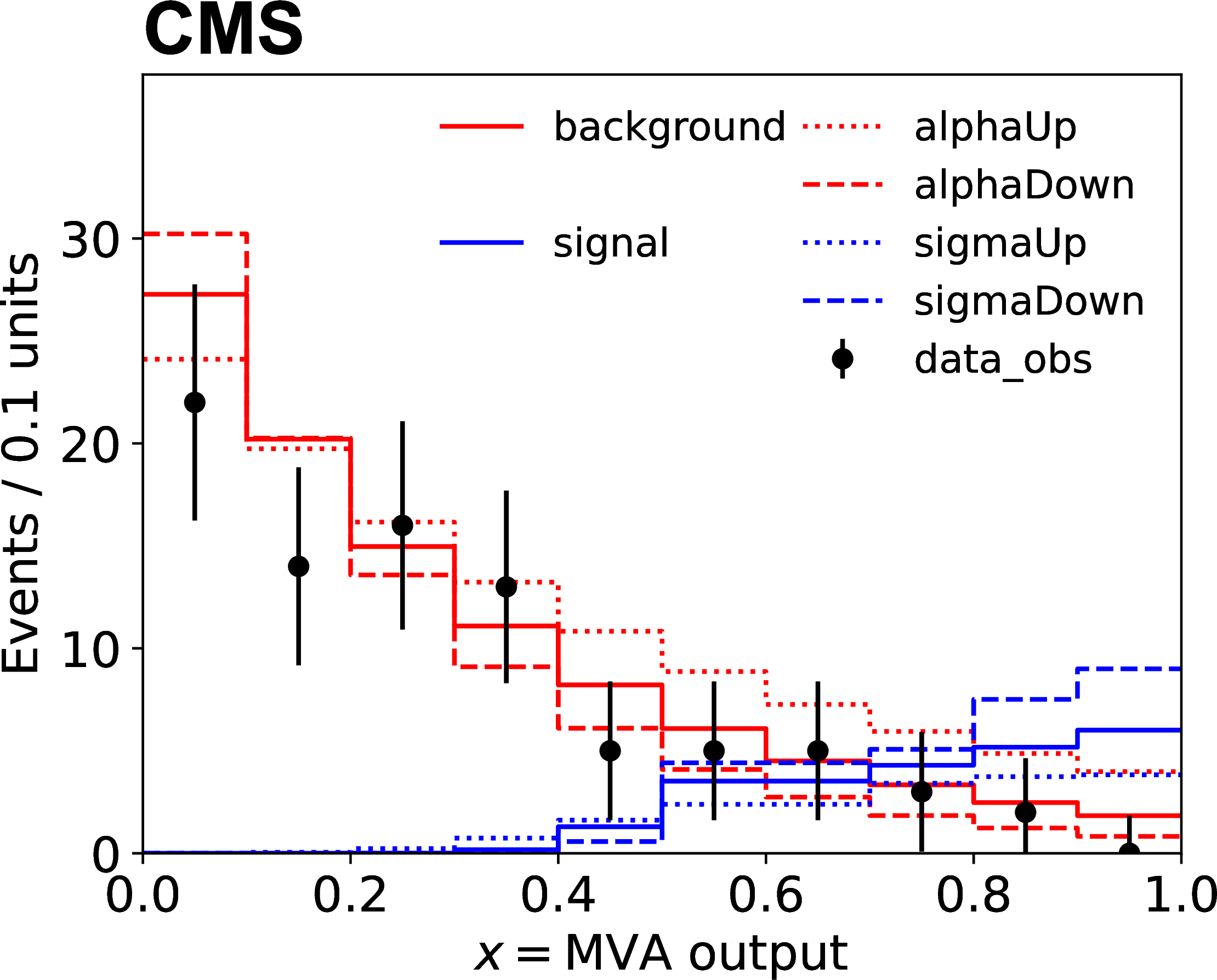
A template-based shape analysis is one in which the observable in each channel is partitioned into \(N_B\) bins. The number of events \(n_b\) in the data that fall within each bin \(b\) (with \(b\) running from 1 to \(N_B\)) is considered as an independent Poisson process. The model becomes a product of Poisson probabilities:
\[p(x;\vec{\mu}, \vec{\nu}) = \prod_{b=1}^{N_B} P(n_b;\lambda (\vec{\mu},\vec{\nu}))\]
In a sense, this is a generalization of the counting analysis. Template shape is the model most used by LHC analyses, as we usually do not know an analytical expression that would describe how our signal or background processes are distributed.
Technically, input to this model is usually given as histograms. Data, backgrounds, signals and variations on backgrounds and signals are all provided as histograms. An example can be seen in the figure below, where sigma and alpha are systematic uncertainties:
Parametric shape analysis
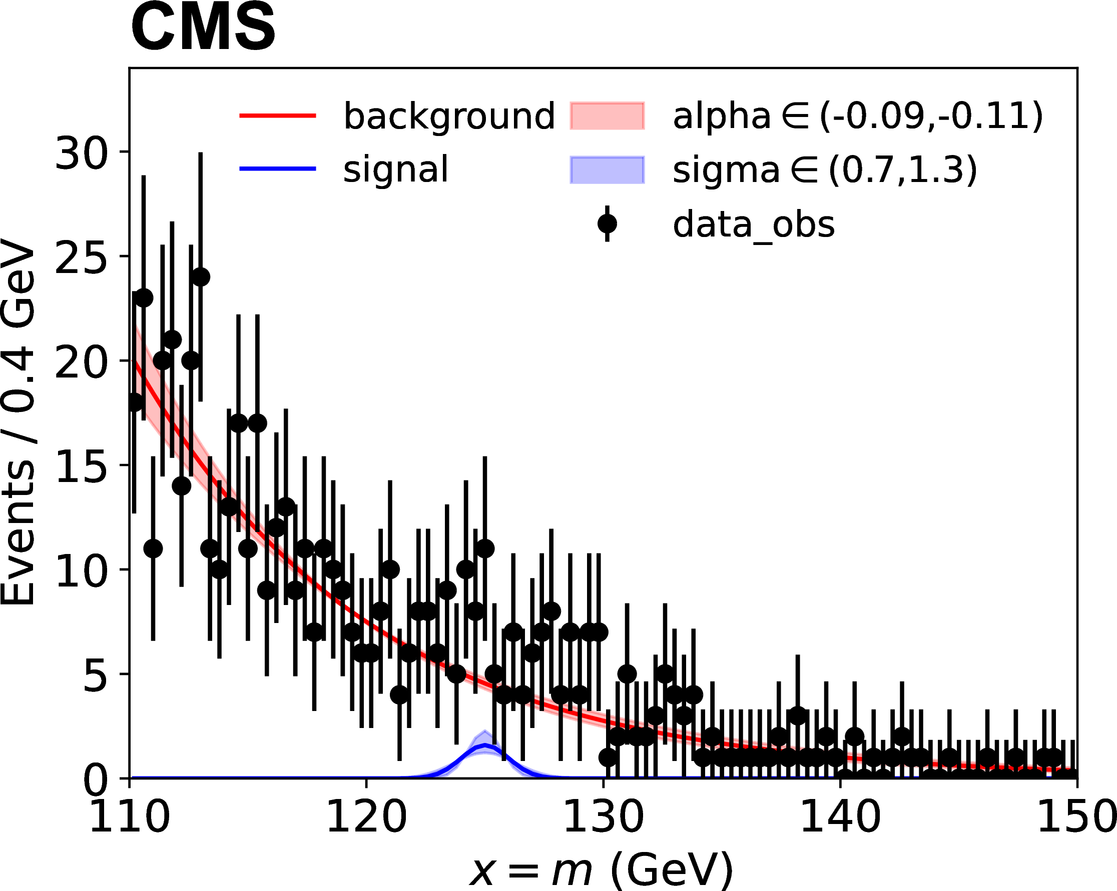
A parametric shape analysis is one that uses analytic functions rather than histograms to describe the probability distributions of continuous primary observables. In these cases, the primary observable \(x\) in each channel can be univariate or multivariate. For example, in the measurements of Higgs boson cross sections in the four-lepton decay mode, the primary observable is bivariate composed of the invariant mass of the four leptons and a kinematic discriminator designed to separate the signal and background processes. The data in parametric shape analyses can be binned, as in the case of template-based analyses, or unbinned. Uncertainties affecting the expected distributions of the signal and background processes can be implemented directly as uncertainties in the parameters of those analytical functions.
\[p(x;\vec{\mu}, \vec{\nu}) = \sum_p \frac{\lambda_p(\vec{\mu},\vec{\nu}) f_p(x; \vec{\mu}, \vec{\nu})}{\sum_p \lambda_p(\vec{\mu}, \vec{\nu})}\]
Here \(p\) stands for process and \(f_p(x; \vec{\mu}, \vec{\nu})\) are the probability density functions for each process. The figure below shows an example, where sigma and alpha are the uncertainties on parameters of the analytic function.
Handling nuisance parameters
When writing the auxiliary component, we usually do not explicitly input the auxiliary data. Instead, we can use priors that encapsulate the knowledge or constraints obtained from the auxiliary data. For example, if auxiliary experiments have measured a nuisance parameter \(\nu\) with a certain mean and uncertainty \(\sigma\), this information can be used to define a prior distribution.
Let’s give a concrete example for luminosity. Imagine a counting analysis, where the primary component is a Poisson. Remember that the number of expected events in that Poisson could be expressed as
\[n_{exp} = \mu \rm{\sigma_{sig}^{eff}} L + \rm{\sigma_{bg}^{eff}} L\]
where \(\mu\) is the signal strength modifier, \(\rm{\sigma_{sig}^{eff}}\) and \(\rm{\sigma_{bg}^{eff}}\) are signal and background effective cross sections and \(L\) is the integrated luminosity. Suppose that, in a different study, we have measured that there is a 2.5% uncertainty on luminosity, which would directly effect the expected number of events:
\[L \rightarrow L(1 + 0.025)^\nu\]
When \(\nu = 0\), no change happens in \(L\), and consequently \(n_{exp}\). When \(\nu = \pm 1\), we have the \(+/-\) effect. We apply a Gaussian constraint as
\[\pi(\nu_0, \nu) = \pi(0 | \nu) - e^{-\frac{1}{2}\nu^2}\]
Hence, the nuisance parameter for luminosity uncertainty is log-normally distributed.
For observed count \(N\), the likelihood becomes
\[\mathcal{L}(\mu, \nu) = \frac{n_{exp}^N e^{-n_{exp}}}{N!}e^{-\frac{1}{2}\nu^2}\]
where
\[n_{exp} = \mu \rm{\sigma_{sig}^{eff}} L \cdot 1.025^\nu + \rm{\sigma_{bg}^{eff}} L \cdot 1.025^\nu\]
In Bayesian analysis, we can marginalize over the nuisance parameters by integrating them out of the posterior distribution. This approach automatically accounts for the uncertainties in the nuisance parameters based on the priors. In frequentist analysis, we can profile out the nuisance parameters by finding the values that maximize the likelihood for each fixed value of the POI.