Content from Introduction to statistical inference
Last updated on 2024-08-01 | Edit this page
Overview
Questions
- What does statistical inference mean?
- What is a statistical model and a likelihood?
- What types of statistical models do we use?
- How do we incorporate constraints on nuisance parameters?
Objectives
- Understand the role of statistical inference in an analysis and related terminology.
- Understand the concept of a statistical model and a likelihood.
- Learn the types of statistical models generally used in analyses.
- Learn how the constraints on nuisance parameters are implemented.
Reference Material
- Combine Manual
- Combine Tutorial at LPC
- Practical Statistics for LHC Physicists - Three CERN Academic Lectures by Harrison Prosper
- Statistics in Theory - A lecture by Bob Cousins
- RooFit - Slides by Wouter Verkerke, one of the RooFit developers
- RooFit Tutorials - A set of macros that showcase all major features of RooFit
- RooStats Manual - A concise, clear, summary of statistics concepts and definitions
- RooStats Tutorial - Tutorial by Kyle Cranmer, one of the RooStats developers
- RooStats Tutorials - A set of macros that showcase all major features of RooStats
- CMS DAS 2014 Statistics Exercise - A tutorial on statistics as used in CMS
- Procedure for the LHC Higgs boson search combination in Summer 2011 - Paper describing LHC statistical procedures
- Combine Github - Github repository for combine
- LPC statistics course - Lectures by Harrison Prosper and Ulrich Heintz, fall 2017
Terminology and Conventions
Here we give pragmatic definitions for a few basic concepts that we will use.
- observable - something you measure in an experiment, for example, a particle’s momentum. Often, a function of measured quantities, for example, an invariant mass of several particles.
- global observable or auxiliary observable - an observable from another measurement, for example, the integrated luminosity.
- model - a set of probability functions (PFs) describing the distributions of observables or functions of observables. The probability functions are called probability density functions (PDFs) if the observables are continuous and probability mass functions (PMF) if the observables are discrete. In the Bayesian approach, the model also includes the prior density.
- model parameter - any variable in your model that is not an observable.
- parameter of interest (POI) - a model parameter of current interest, for example, a cross section.
- nuisance parameter - every model parameter other than your parameter (or parameters) of interest.
- data or data set - a set of values of observables, either measured in an experiment or simulated.
- likelihood - a model computed for a particular data set.
- hypothesis - a model in which all quantities are specified: observables, model parameters, and prior PDFs (in case of Bayesian inference).
- prior - a probability or probability density for an observable or a model parameter that is independent of the data set. Priors are a key feature of Bayesian inference. However, priors can be used in frequentist inference only if they can be interpreted as relative frequencies.
- Bayesian - a school of statistical inference based on the likelihood and a prior.
- frequentist - a school of statistical inference based on the likelihood only.
Statistical inference is the last step of an analysis and plays a crucial role in interpreting the experimental data. It involves using statistical methods to draw conclusions about the underlying physical processes based on observed data. This process includes defining a statistical model, constructing a likelihood function, and employing techniques such as hypothesis testing and parameter estimation to extract meaningful insights. Let’s start with the concept of a statistical model.
Statistical model
Statistical model is the mathematical framework used to describe and make inferences about the underlying processes that generate observed data. It encodes the probabilistic dependence of the observed quantities (i.e. data) on parameters of the model. These parameters are not directly observable but can be inferred from experimental data. They include
- parameters of interest (POI), \(\vec{\mu}\): The quantities we are interested in estimating or testing. Examples are cross section, signal strength modifier, resonance mass, …
- nuisance parameters, \(\vec{\nu}\): parameters that are not of direct interest, but required to explain data. These could be uncertainties of experimental or theoretical origin, such as detector effects, background measurements, lumi calibration, cross-section calculation.
Data are also partitioned into two:
- primary observables, \(\vec{x}\): Appear in components of the model that contain the POIs.
- auxiliary observables, \(\vec{y}\): Appear only in components of the model that contain the nuisance parameters.
Likelihood is the value of the statistical model at a given fixed set of data as a function of parameters.
Statistical model provides the complete mathematical description of an analysis and is the starting point of any interpretation.
Now let’s express this mathamatically. Our statistical model be described as \(p(\rm{data,\vec{\Phi}})\) where \(\vec{\Phi}\) are the model parameters. For the sake of numerical efficiency, we can factorize it into two parts:
\[p(\vec{x},\vec{y};\vec{\Phi}) = p(\vec{x};\vec{\mu},\vec{\nu}) \prod_k p_k(\vec{y}_k;\vec{\nu}_k)\]
- primary component: \(p(\vec{x};\vec{\mu},\vec{\nu})\). Relates POI to primary observables.
- auxiliary component: \(\prod_k p_k(\vec{y}_k;\vec{\nu}_k)\). Constrains nuisance parameters.
Likelihood function is constructed by evaluating \(p(\rm{data,\vec{\Phi}})\) on a dataset:
\[L(\vec{\Phi}) = \prod_d p(\vec{x}_d;\vec{\mu},\vec{\nu}) \prod_k p_k(\vec{y}_k;\vec{\nu}_k)\]
where \(d\) runs over all entries in data.
This likelihood can be used in both frequentist and Bayesian calculations.
Types of statistical models
Counting analysis
A counting analysis is one for which the statistical model has only one primary observable, namely the total event count in a single channel that includes multiple sources of signal and background. In the following, the primary observable is labeled \(n\). The probability to observe \(n\) events is described by a Poisson distribution,
\[p(n;\lambda(\vec{\mu}, \vec{\nu})) =\lambda^n\frac{e^{-\lambda}}{n!}\]
where the expected value, \(\lambda\), can be a function of one or more parameters, and represents the total number of expected signal and background events.
For our analyses, we usually express \(\lambda\), the expected number of events as:
\[\lambda \equiv n_{exp} = \mu \rm{\sigma_{sig}^{eff}} L + \rm{\sigma_{bg}^{eff}} L\]
Here \(\rm{\sigma_{sig}^{eff}}\) and \(\rm{\sigma_{bg}^{eff}}\) are signal and background effective cross sections (i.e. cross section times selection efficiency times detector acceptance) and \(L\) is the integrated luminosity. Our parameter of interest here is \(\mu\), the signal strength modifier. The estimated value of \(\mu\) would be able to tell us if the signal is discovered, excluded or still out of reach.
Template shape analysis
A shape analysis is defined as one that incorporates one or more primary observables, beyond a single number of events.
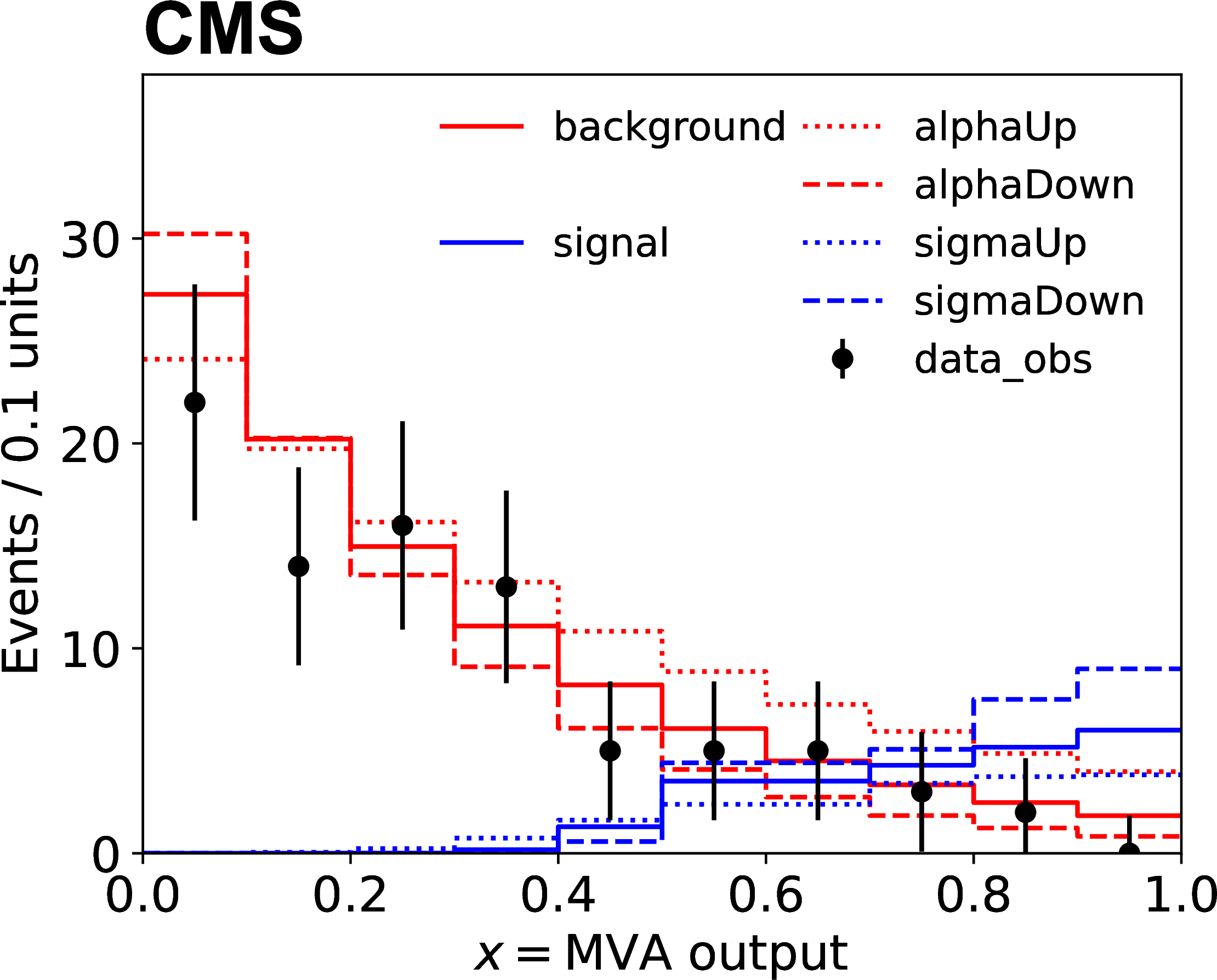
A template-based shape analysis is one in which the observable in each channel is partitioned into \(N_B\) bins. The number of events \(n_b\) in the data that fall within each bin \(b\) (with \(b\) running from 1 to \(N_B\)) is considered as an independent Poisson process. The model becomes a product of Poisson probabilities:
\[p(x;\vec{\mu}, \vec{\nu}) = \prod_{b=1}^{N_B} P(n_b;\lambda (\vec{\mu},\vec{\nu}))\]
In a sense, this is a generalization of the counting analysis. Template shape is the model most used by LHC analyses, as we usually do not know an analytical expression that would describe how our signal or background processes are distributed.
Technically, input to this model is usually given as histograms. Data, backgrounds, signals and variations on backgrounds and signals are all provided as histograms. An example can be seen in the figure below, where sigma and alpha are systematic uncertainties:
Parametric shape analysis
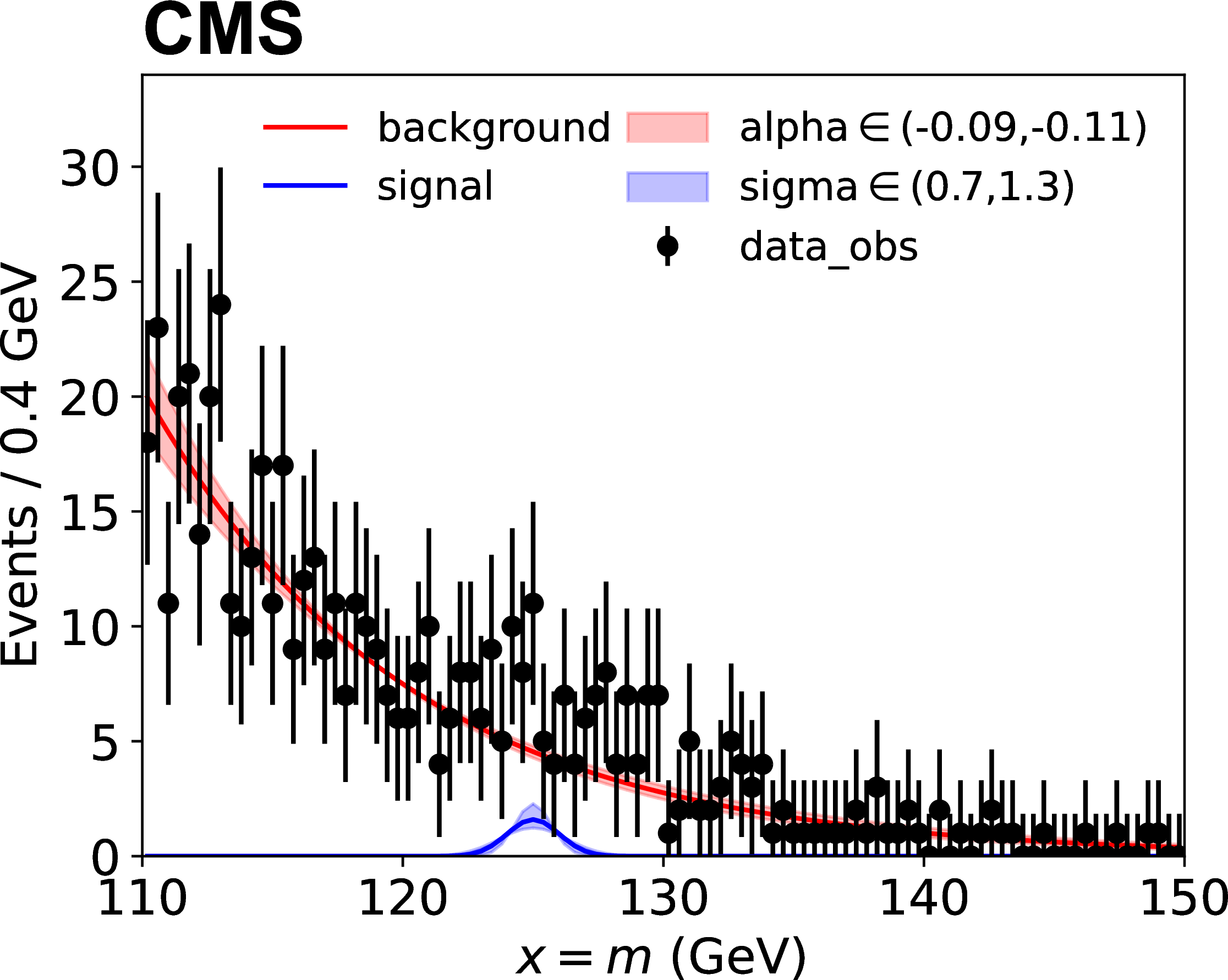
A parametric shape analysis is one that uses analytic functions rather than histograms to describe the probability distributions of continuous primary observables. In these cases, the primary observable \(x\) in each channel can be univariate or multivariate. For example, in the measurements of Higgs boson cross sections in the four-lepton decay mode, the primary observable is bivariate composed of the invariant mass of the four leptons and a kinematic discriminator designed to separate the signal and background processes. The data in parametric shape analyses can be binned, as in the case of template-based analyses, or unbinned. Uncertainties affecting the expected distributions of the signal and background processes can be implemented directly as uncertainties in the parameters of those analytical functions.
\[p(x;\vec{\mu}, \vec{\nu}) = \sum_p \frac{\lambda_p(\vec{\mu},\vec{\nu}) f_p(x; \vec{\mu}, \vec{\nu})}{\sum_p \lambda_p(\vec{\mu}, \vec{\nu})}\]
Here \(p\) stands for process and \(f_p(x; \vec{\mu}, \vec{\nu})\) are the probability density functions for each process. The figure below shows an example, where sigma and alpha are the uncertainties on parameters of the analytic function.
Handling nuisance parameters
When writing the auxiliary component, we usually do not explicitly input the auxiliary data. Instead, we can use priors that encapsulate the knowledge or constraints obtained from the auxiliary data. For example, if auxiliary experiments have measured a nuisance parameter \(\nu\) with a certain mean and uncertainty \(\sigma\), this information can be used to define a prior distribution.
Let’s give a concrete example for luminosity. Imagine a counting analysis, where the primary component is a Poisson. Remember that the number of expected events in that Poisson could be expressed as
\[n_{exp} = \mu \rm{\sigma_{sig}^{eff}} L + \rm{\sigma_{bg}^{eff}} L\]
where \(\mu\) is the signal strength modifier, \(\rm{\sigma_{sig}^{eff}}\) and \(\rm{\sigma_{bg}^{eff}}\) are signal and background effective cross sections and \(L\) is the integrated luminosity. Suppose that, in a different study, we have measured that there is a 2.5% uncertainty on luminosity, which would directly effect the expected number of events:
\[L \rightarrow L(1 + 0.025)^\nu\]
When \(\nu = 0\), no change happens in \(L\), and consequently \(n_{exp}\). When \(\nu = \pm 1\), we have the \(+/-\) effect. We apply a Gaussian constraint as
\[\pi(\nu_0, \nu) = \pi(0 | \nu) - e^{-\frac{1}{2}\nu^2}\]
Hence, the nuisance parameter for luminosity uncertainty is log-normally distributed.
For observed count \(N\), the likelihood becomes
\[\mathcal{L}(\mu, \nu) = \frac{n_{exp}^N e^{-n_{exp}}}{N!}e^{-\frac{1}{2}\nu^2}\]
where
\[n_{exp} = \mu \rm{\sigma_{sig}^{eff}} L \cdot 1.025^\nu + \rm{\sigma_{bg}^{eff}} L \cdot 1.025^\nu\]
In Bayesian analysis, we can marginalize over the nuisance parameters by integrating them out of the posterior distribution. This approach automatically accounts for the uncertainties in the nuisance parameters based on the priors. In frequentist analysis, we can profile out the nuisance parameters by finding the values that maximize the likelihood for each fixed value of the POI.
Content from Limits
Last updated on 2024-08-01 | Edit this page
Overview
Questions
- What are limits?
- What are expected and observed limits?
- How do we calculate limits?
Objectives
- Understand the concept of limits, expected limits, and observed limits.
- Familiarize with the steps of calculating limits.
- Familiarize with the concepts of hypothesis testing, test statistic, p-values and confidence level.
What are limits?
Limits are constraints placed on the parameters of a theoretical model based on the experimental data. They help determine the range within which new particles or interactions could exist.
Observed limits: These are limits derived directly from the experimental data. They represent the actual constraint on the parameter of interest based on the measurements taken during the experiment.
Expected limits: These are limits based on simulated data assuming no new phenomena exist (i.e., that the null hypothesis is true). They provide a benchmark for comparing the observed limits to what would be expected if only known physics were at play.
Calculating limits
The process of calculating limits typically involves the following steps:
Define the statistical model and construct the likelihood :
-
Perform Hypothesis Testing:
- Null hypothesis (or background-only hypothesis) (\(H_0\)): This hypothesis assumes that there is no new physics, meaning the data can be fully explained by the standard model or another established theory.
- Alternative hypothesis or signal+background hypothesis (\(H_1\)): This hypothesis posits the presence of new physics, implying deviations from the predictions of the null hypothesis.
- Test statistic: Calculate a test statistic, such as the profile likelihood ratio, which compares how well the data fits under both \(H_0\) and \(H_1\). The profile likelihood ratio is defined as: \[\lambda(\mu) = \frac{\mathcal{L}(\mu, \hat{\nu}(\mu))}{\mathcal{L}(\hat{\mu}, \hat{\nu})}\]: where \(\mathcal{L}\) is the likelihood function, \(\mu\) and \(\nu\) represent the parameters of interest and nuisance parameters, \(\hat{\mu}\) and \(\hat{\nu}\) are the best-fit parameters, and \(\hat{\nu}(\mu)\) is the conditional maximum likelihood estimator of the nuisance parameters given \(\mu\). Note that in the current LHC analyses, we use more complex test statistics such as the LHC-style test statistic. However, despite the added complexity, the main idea is the same. The test statistic is evaluated for observed data or pseudo-data
- p-value: Determine the p-value, which quantifies the probability of obtaining data as extreme as observed under the null hypothesis. A small p-value indicates that the null hypothesis is unlikely.
- Confidence level: Set a confidence level (e.g., 95%) to determine the exclusion limits. The confidence level represents the probability that the true parameter values lie within the calculated limits if the experiment were repeated many times.
-
Calculate limits: The p-values for the signal-only and signal+BG hypotheses are combined in a certain way to obtain limits. At the LHC, we use the so-called \(\mathrm{CL_s}\) quantity.
- Expected limits: Obtain by comparing observed data with 1) signal MC + estimated BG and 2) with only estimated BG. Observed limits check the consistency of the observation with the signal + BG hypothesis and compares it to the BG-only hypothesis.
- Expected limits: Get the null hypothesis, e.g. background estimation from simulation or a data-driven method. Obtain the limits by comparing estimated BG with signal + estimated BG. Useful for predicting the analysis sensitivity.
-
Compare and interpret:
- Compare the observed limits with the expected limits to interpret the results. If the observed limits are significantly different from the expected limits, this may indicate potential new physics.
Content from The CMS Combine statistical analysis and combination software
Last updated on 2024-08-01 | Edit this page
Overview
Questions
- What is Combine?
- How do I input a statistical model into Combine?
- What tasks does Combine perform?
- Can I use Combine outside CMS? Where can I find detailed documentation?
- What does it mean to publish a statistical model, and why is it so important?
Objectives
- Get introduced to the Combine tool.
- Learn the principles of how to input a statistical model
- Learn the set of tasks performed by Combine.
- Learn how to access information on how to run Combine outside CMS, and access documentation.
- Learn the concept of statistical model publication and how to access the first model published by CMS.

What is Combine?
Combine is the statistical analysis software used in CMS, built around the ROOT, RooFit and RooStats packages. It provides a command-line interface to several common workflows used in HEP statistical analysis. Combine provides a standardized access to these workflows, which makes it a very practical and reliable tool. As of 2024, more than 90% of the analyses in CMS use Combine for statistical inference.
Models and the datacard
Combine implements the statistical model and the corresponding likelihood in a RooFit-based custom class. The inputs to the model are encapsulated in a human-readable configuration file called the datacard. Datacard includes information such as
- signal and background processes, shapes and rates
- systematic and statistical uncertainties incorporated as nuisance parameters and their effects on the rates, along with their correlations
- multiplicative scale factors that modify the rate of a given process in a given channel
Combine supports building models for counting analyses, template shape analyses and parametric shape analyses. Though the main datacard syntax is similar for these three cases, there are minor differences reflecting the model input. For example, in the case for a template shape model, one needs to specify a ROOT file with input histograms, and in the case of a parametric shape model, one needs to specify the process probability distribution functions.
Constructing a datacard is usually the level most users input information to Combine. However, there are some cases where the statistical model requires modifications. An example case is where we need a model with multiple parameters of interest associated with different signal processes (e.g. measurement of signal strength modifiers for two different Higgs production channels, gluon-gluon fusion and vector boson fusion). Combine also allows to build custom models by introducing modified model classes. Combine scales well with model complexity, and therefore is a powerful tool for combining a large number of analyses.
Tasks performed by Combine
Combine is capable of performing many statistical tasks. The main interface is with the command below
combine <datacard.[txt|root]> -M <method>where one enters a datacard (either as text or in a ROOT-converted format) and specifies the method pointing to a task.
Here is a set of methods used for extracting results:
- HybridNew: compute modified frequentist limits with pseudo-data, p-values, significance and confidence intervals with several options, –LHCmode LHC-limits is the recommended one.
- AsymptoticLimits: limits calculated according to the asymptotic formulas in arxiv:1007.1727, valid for large event counts.
- Significance: simple profile likelihood approximation for calculating significances.
- BayesianSimple: and MarkovChainMC compute Bayesian upper limits and credible intervals for simple and arbitrary models.
- MultiDimFit: perform maximum likelihood fit, with multiple POIs, estimate CI from likelihood scans.
Combine also provides an extensive toolset for validation and diagnosis:
- GoodnessOfFit: perform a goodness of fit test for models including shape information using several GoF estimators (saturated, Kolmogorov-Smirnov, Anderson-Darling)
- Impacts: evaluate the shift in POI from  variation for each nuisance parameter.
- ChannelCompatibiltyCheck: check how consistent are the individual channels of a combination are
- GenerateOnly: generate random or Asimov pseudo-datasets for use as input to other methods
Running Combine and detailed references
In 2024 Combine tool became available to the public along with
- a detailed paper: CMS-CAT-23-001 / arXiv:2404.06614 and a
- detailed user manual: Combine github pages
The easiest way to run Combine is to use a Docker containerized version of it (as we will do in the next exercise). The container can be installed as:
docker run --name combine -it gitlab-registry.cern.ch/cms-cloud/combine-standalone:<tag>where <tag> should be replaced by the latest tag,
which is currently v9.2.1
There are also other ways, e.g. based on Conda or a standalone compilation. All instructions are given in this documentation.
Publishing statistical models
Statistical models of our numerous physics analyses would provide an
excellent resource for the community.
Publishing them will help maximize the scientific impact of the
analyses, and facilitate
- Preservation and documentation: the mathematical construction of the analysis in full detail.
- Combination of multiple analyses
- Reinterpretation and reuse (within and outside the collaborations):
- Education on statistics procedures
- Tool development: Statistical software updates can use real world examples to test and debug their recent developments.
- One can certainly find other use cases!
The community report “Publishing statistical models: Getting the most out of particle physics experiments”, SciPost Phys. 12, 037 (2022), arXiv:2109.04981 makes the scientific case for statistical model publication, and discuss technical developments.
In December 2023, CMS Collaboration took the decision to release statistical models for all forthcoming analyses by default. This is in accordance with open access policy of CERN and the FAIR principles (findable, accessible, interoperable, reusable).
The first statistical model published is that for the Higgs boson discovery. The model consists of the Run 1 combination of 5 main Higgs channels (CMS-HIG-12-028). The model can be found in this link.
You can download the model into the Combine container and see the discovery for yourself. The commands are available to combine channels, calculate the significance, measure the signal strength modifier and build a model as Higgs-vector boson, Higgs-fermion coupling modifiers as POIs.
More models are on their way to become public soon!
Content from Limit calculation challenge
Last updated on 2024-08-01 | Edit this page
Overview
Questions
- How do I write a Combine datacard for a counting analysis and for a shape analysis?
- How do I incorporate the effects of systematic uncertainties?
- How do I calculate expected and observed limits?
- How do I interpret the resulting limits?
Objectives
- Construct a Combine datacard for a counting analysis, learn to modify systematics.
- Construct a Combine datacard for a shape analysis, learn to modify systematics.
- Calculate limits using Combine with different methods for counting and shape datacards and compare.
- Understand what the limits mean.
The goal of this exercise is to use the Combine tool to
calculate limits from the results of the \(Z'\) search studied in the previous
exercises. We will use the Zprime_hists_FULL.root file
generated during the Uncertainties
challenge. We will build various datacards from it, add systematics,
calculate limits on the signal strength modifier and understand the
output.
Prerequisite
For the activities in this session you will need:
- Your Combine docker container (installation instructions provided in the setup section of this tutorial)
Statistical analysis as a counting experiment
At the end of the https://cms-opendata-workshop.github.io/workshop2024-lesson-event-selection/,
you applied a set of selection criteria to events that would enhance
\(Z'\) signal from SM backgrounds.
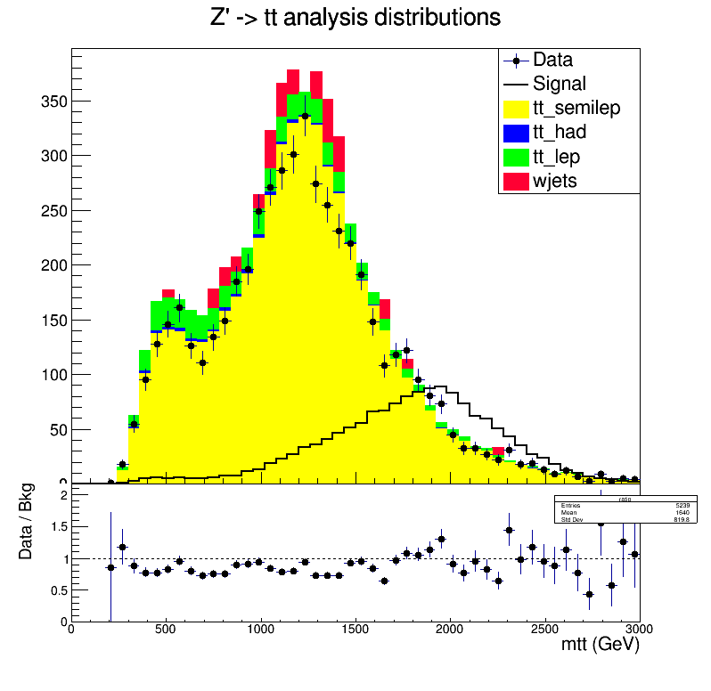
Then you obtained the ttbar mass distributions for data, \(Z'\) signal and a set of SM background
processes after this selection. In the Uncertainties
challenge exercise, you learned to obtain variations on these
distributions arising from certain systematic effects. In this first
exercise, we will treat the events surviving the selection as a single
quantity to perform a statistical analysis on a counting experiment. In
other words, we will collapse the mtt distributions into a
single “number of events” by integrating over all bins. Then we will use
these numbers obtained for all histograms, including those with
systematic variations, to build a counting experiment datacard.
First, start your Combine Docker container and make a working directory:
Download the Zprime_hists_FULL.root and the python
script to make the datacard:
BASH
wget https://github.com/cms-opendata-workshop/workshop2024-lesson-statistical-inference/raw/main/instructors//Zprime_hists_FULL.root
wget https://github.com/cms-opendata-workshop/workshop2024-lesson-statistical-inference/raw/main/instructors//writecountdatacard.py
You can look into the writecountdatacard.py script to
see how the datacard is written from the ROOT file. Run the script:
(ignore the output for the moment). Now look into
datacard_counts.txt and try to answer the following
questions:
Questions
- Which is the background contributing most?
- What can you say when you compare data, total backgrounds, and signal counts?
- Can you understand the effect of the various systematic uncertainties?
- Which systematic is expected to have the overall bigger impact?
- Which process is affected most by systematics?
Now run Combine over this datacard to obtain the limits on our
parameter of interest, signal strength modifier, with the simple
AsymptoticLimits option:
You will see some error messages concerning the computation of the observed limit, arising from numerical stability issues. In order to avoid this, let’s rerun by limiting the signal strength modifier to be maximum 2:
Look at the output, and try to answer the following:
Questions
- What is the observed limit? What is the expected limit? What are the uncertainties on the expected limit?
- Did our analysis exclude this particular \(Z'\) signal?
- What can you say when you compare the values of the observed limit with the expected limit?
- What does it mean that the observed limit is much lower compared to the expected limit? Does this make sense? Hint: Go back to the datacard and look at the data, background and signal counts.
Taming the observed (DON’T TRY THIS AT HOME!)
A hypothetical question: What would bring the observed limit within the expected uncertainties? Do the necessary modifications in the datacard and see if the limit behaves as you predicted.
You can rerun writecountdatacard.py to reset the
datacard.
Observed limit is below the expected boundaries because we have much more MC compared to data. This means there is less room for signal to be accommodated in data, i.e. excluding signal becomes easier. If we had more data, or less backgrounds, there would be more room for signal, and the observed limit would be more consistent with the expected. So hypothetically one could
- Increase the data counts, or
- Decrease counts in one or more background processes.
The point of this question was to increase the understanding. We never do this in real life!!!
Add uncertainties to the datacard
Now let’s add more uncertainties, both systematic and statistical. Let’s start with adding a classic - the systematic uncertainty due to luminosity measurement:
Challenge: Add a lognormal luminosity systematic
- Please add a lognormal systematic uncertainty on luminosity (called
lumi) that affects all signal and background processes, inducing a symmetric 2.5% up and down variation. - Run Combine with the new datacard and discuss the effect on the limits.
lumi lnN 1.025 1.025 1.025 1.025 1.025Now let’s add a statistical uncertainty. Our signal and background yields come from Monte Carlo, and the number of events could be limited, resulting on non-negligible statistical uncertainties. We apply event weights to these MC events so that the resulting rate matches a certain value, e.g. cross section times the luminosity. Statistical uncertainties are particularly relevant if both the yields are small and the event weights are large (i.e. much less actual MC events are available compared to the expected yield). Here is a quote from the Combine documentation on how to take these into account:
“gmN stands for Gamma, and is the recommended choice for the statistical uncertainty in a background determined from the number of events in a control region (or in an MC sample with limited sample size). If the control region or simulated sample contains N events, and the extrapolation factor from the control region to the signal region is α, one shoud put N just after the gmN keyword, and then the value of α in the relevant (bin,process) column. The yield specified in the rate line for this (bin,process) combination should equal Nα.”
Now let’s get back to the output we got from running
writecountdatacard.py. There you see the number of total
unweighted events, total weighted events and event weight for each
process.
Challenge: Add a statistical uncertainty
Look at the output of writecountdatacard.py:
- Which process has the largest event weight?
- Can you incorporate the statistical uncertainty for that particular process to the datacard?
- Run Combine and discuss the effect on the limits.
- OPTIONAL: You can add the statistical uncertainties for the other processes as well and observe their effect on the limits.
stat_signal     gmN 48238  0.0307         -              -              -              -
stat_tt_semilep gmN 137080 -              0.0383         -              -              -
stat_tt_had     gmN 817    -              -              0.0636         -              -
stat_tt_lep     gmN 16134  -              -              -              0.0325         -
stat_wjets	gmN 19     -              -              -              -              15.1623
Improve the limit
Improving the limit
What would you do to improve the limit here?
Hint: Look at the original plot displaying the data, background and signal distributions.
- In a count experiment setup, we can consider taking into account a
part of the
mttdistribution where the signal is dominant. - We can do a shape analysis, which takes into account each bin separately.
Let’s improve the limit in the couting experiment setup by computing total counts considering only the last 25 bins out of the 50 total:
We also added flags to automatically add the satistical and lumi uncertainties :). How did the yields change? Did the limit improve? You can try with different starting bin options to see how the limits change.
Shape analysis
Now we move to a shape analysis, where each bin in the
mtt distribution is taken into account. Datacards for shape
analyses are built with similar principles as those for counting
analyses, but their syntax is slightly different. Here is the shape
datacard for the \(Z'\)
analysis:
BASH
wget https://github.com/cms-opendata-workshop/workshop2024-lesson-statistical-inference/raw/main/instructors/datacard_shape.txtExamine it and note the differences in syntax. To run on Combine,
this datacard needs to be accompanied by the
Zprime_hists_FULL.root file, as the shapes are directly
retrieved from the histograms within.
Run Combine with this datacard. How do the limits compare with respect to the counts case?
Limits on cross section
So far we have worked with limits on the signal strength modifier. How can we compute the limits on cross section? Can you calculate the upper limit on \(Z'\) cross section for this model?
We can multiply the signal strength modifier limit with the theoretically predicted cross section for the signal process.