Content from Introduction
Last updated on 2024-07-02 | Edit this page
Estimated time: 5 minutes
Overview
Questions
- What is C++?
- What is ROOT?
- What is the point of these exercises?
Objectives
- Learn a bit about C++ and how to compile C++ code.
- Learn how to use ROOT to write and read from files, using the C++ libraries.
- Learn how to use ROOT to investigate data and create simple histograms.
- Explore the ROOT python libraries.
Let’s talk about ROOT!
From the ROOT website:
Testimonial
ROOT is a framework for data processing, born at CERN, at the heart of the research on high-energy physics. Every day, thousands of physicists use ROOT applications to analyze their data or to perform simulations.
In short, ROOT is an overarching toolkit that defines a file structure, methods to analyze particle physics data, visualization tools, and is the backbone of many widely used statistical analysis tool kits, such as RooFit and RooStats. You don’t need to use ROOT for your own analysis, but you will have to have some familiarity with it when you are first accessing the open data.
OK, that sounds cool. So what’s the deal with C++?
ROOT and C++
In the mid-80’s, C++ extended the very popular C programming language, primarily with the introduction of object-oriented programming (OOP). This programming paradigm was adopted by many particle physics experiments in the 1990’s and when ROOT was written, it was written in C++. While there are now python hooks to call the ROOT functions, the underlying code is all in C++.
Because C++ is a compiled code, it is usually much faster than a scripted language like python, though that is changing with modern python tools. Still, since much of the original analysis and access code was written in C++ and calling the C++ ROOT libraries, it’s good to know some of the basics of ROOT, in a C++ context.
Most CMS analysts interface with ROOT using python scripts and you may find yourself using a similar workflow. Later on in this lesson, we’ll walk you through some very basic python scripts and point you toward more in-depth tutorials, for those who want to go further.
You still have choices!
Just to emphasize, you really only need to use ROOT and C++ at the early stages of analyzing CMS Open Data in the AOD (Run 1) or MiniAOD (Run 2) formats. These datasets require using CMS-provided tools that perform much better in C++ than python. However, downstream in your analysis or to analyze Run 2 NanoAOD files, you are welcome to use whatever tools and file formats you choose.
Key Points
- C++ has a reputation for being intimidating, but there are only a few things you need to learn to edit the open data code for your own uses.
- You can use the ROOT toolkit using both C++ and python.
- Some ROOT code is written in C++ to access the datafiles.
- People will often use simpler C++ scripts or python scripts to analyze reduced datasets.
Content from Lightning overview of C++
Last updated on 2024-07-09 | Edit this page
Estimated time: 15 minutes
Overview
Questions
- How do I write and execute C++ code?
Objectives
- To write a hello-world C++ program
Setting up your working area
If you completed the Docker pre-exercises you should already have worked through this episode, under Download the docker images for ROOT and python tools and start container, and you will have
- a working directory
cms_open_data_rooton your local computer - a docker container with name
my_rootcreated with the working directorycms_open_data_rootmounted into the/codedirectory of the container.
Start your ROOT container with
In the container, you will be in the /code directory and
it shares the files with your local cms_open_data_root
directory.
If you’re using apptainer:
Whenever you see a docker start instruction, replace it
with apptainer shell to open either the ROOT or Python
container image. The specific commands in this pre-exercise and during
the live workshop will be given for docker, since that is the most
common application. As a general rule, editing of files will be done in
the standard terminal (the containers do not have all text editors!) or
via the jupyter-lab interface, and then commands will be executed inside
the container shell. If you see Singularity> on your
command line, you are ready to run a ROOT or python script.
Your first C/C++ program (Optional Review!)
Let’s start with writing a simple hello world program in
C. First we’ll edit the source code with an editor of your
choice.
Note that you will edit the file in a local terminal on your
computer and then run the file in the Docker environment. This
is because we mounted the cms_open_data_root directory on
your local disk such that it is visible inside the Docker container.
Let’s create a new file called hello_world.cc in the
cms_open_data_root directory, using your preferred
editor.
The first thing we need to do, is include some standard
libraries. These libraries allow us to access the C and C++ commands to
print to the screen (stdout and stderr) as
well as other basic function.
At the very beginning of your file, add these three lines
The first library, cstdlib, you will see in almost every
C++ program as it has many of the very basic functions, including those
to allocate and free up memory, or even just exit the program.
The second library, cstdio, contains the basic C
functions to print to screen, like printf.
The third library, iostream, contains C++ functions to
print to screen or write to files.
Usually people will use one or the other of the C or C++ printing functions, but for pedagogical purposes, we show you both.
Every C++ program must have a main function. So let’s
define it here. The scope of this function is defined by curly brackets
{ }. So let’s add
The int at the beginning tells us that this function
will be returning an integer value. At the end of the main
function we have return 0, which usually means the function
has run successfully to completion.
Warning!
Note that at the end of return 0, we have a semicolon
;, which is how C/C++ programs terminate lines. If you’re
used to programming in python or any other language that does not use a
similar terminator, this can be tough to remember. If you get errors
when you compile, check the error statements for the lack of
; in any of your lines!
For this function, we are not passing in any arguments so we just
have the empty ( ) after the main.
This function would compile, but it doesn’t do anything. Let’s print
some text to screen. Before the return 0; line, let’s add
these three lines.
CPP
printf("Hello world! This uses the ANSI C 'printf' statement\n");
std::cout << "Hello world! This uses the C++ 'iostream' library to direct output to standard out." << std::endl;
std::cerr << "Hello world! This uses the C++ 'iostream' library to direct output to standard error." << std::endl;The text itself, should explain what they are doing. If you want to learn more about standard error and standard output, you can read more on Wikipedia.
OK! Your full hello_world.cc should look like this.
CPP
#include <cstdlib>
#include <cstdio>
#include <iostream>
int main() {
printf("Hello world! This uses the ANSI C 'printf' statement\n");
std::cout << "Hello world! This uses the C++ 'iostream' library to direct output to standard out." << std::endl;
std::cerr << "Hello world! This uses the C++ 'iostream' library to direct output to standard error." << std::endl;
return 0;
}This won’t do anything yet though! We need to compile the
code, which means turning this into machine
code. To do this, we’ll use the GNU C++ compiler,
g++. Once you have saved your file, go to the container
shell, make sure (e.g. with ls -l) that you your file is in
the current directory and type this in your shell.
This compiles your code to an executable called
hello_world. You can now run this by typing the following
on the shell command line, after which you’ll see the subsequent
output.
OUTPUT
Hello world! This uses the ANSI C 'printf' statement
Hello world! This uses the C++ 'iostream' library to direct output to standard out.
Hello world! This uses the C++ 'iostream' library to direct output to standard error.When you are working with the Open Data, you will be looping over events and may find yourself making selections based on certain physics criteria. To that end, you may want to familiarize yourself with the C++ syntax for loops and conditionals.
Key Points
- We must compile our C++ code before we can execute it.
Content from Using ROOT with C++ to write and read a file
Last updated on 2024-07-09 | Edit this page
Estimated time: 35 minutes
Overview
Questions
- Why do I need to use ROOT?
- How do I use ROOT with C++?
Objectives
- Write a ROOT file using compiled C++ code.
- Read a ROOT file using compiled C++ code.
Why ROOT?
HEP data can be challenging! Not just to analyze but to store! The data don’t lend themselves to neat rows in a spreadsheet. One event might have 3 muons and the next event might have none. One event might have 2 jets and the next event might have 20. What to do???
The ROOT toolkit provides a file format that can allow for efficient storage of this type of data with heterogenous entries in each event. It also provides a pretty complete analysis environment with specialized libraries and visualization packages. Until recently, you had to install the entire ROOT package just to read a file. The software provided by CMS to read the open data relies on some minimal knowledge of ROOT to access. From there, you can write out more ROOT files for further analysis or dump the data (or some subset of the data) to a format of your choosing.
Interfacing with ROOT
ROOT is a toolkit. That is, it is a set of functions and libraries that can be utilized in a variety of languages and workflows. It was originally written in C++ and lends itself nicely to being used in standard, compiled C++ code.
However, analysts wanted something more interactive, and so the ROOT
team developed CINT,
a C++ interpreter. This gave users an iteractive environment where
they could type of C++ code one line at a time and have it executed
immediately. This gave rise to C++ scripts that many analysts use and in
fact the sample ROOT
tutorals are almost exclusively written as these C++ scripts (with a
.C file extension). Because they are written to run in
CINT, they usually do not need the standard C++ include
statements that you will see in the examples below.
With the rise of the popularity of python, a set of Python-C++ bindings were written and eventually officially supported by the ROOT development team, called PyROOT. Many analysts currently write the code which plots or fits their code using PyROOT, and we will show you some examples later in this exercise.
What won’t you learn here
ROOT is an incredibly powerful toolkit and has a lot in it. It is heavily used by most nuclear and particle physics experiments running today. As such, a full overview is beyond the scope of this minimal tutorial!
This tutorial will not teach you how to:
- Make any plots more sophisticated than a basic histogram.
- Fit your data
- Use any of the HEP-specific libraries
(e.g.
TLorentzVector)
OK, where can I learn that stuff?
There are some great resources and tutorials out there for going further.
- The official ROOT Primer. The recommended starting point to learn what ROOT can do.
- The official ROOT tutorials This is a fairly comprehensive listing of well-commented examples, written in C++ scripts that are designed to be run from within the ROOT C-interpreter.
- ROOT tutorial (2022).. Tutorial from offical ROOT project for summer students.
- Efficient analysis with ROOT. This is a more complete, end-to-end tutorial on using ROOT in a CMS analysis workflow. It was created in 2020 by some of our CMS colleagues for a separate workshop, but much of the material is relevant for the Open Data effort. It takes about 2.5 hours to complete the tutorial.
- ROOT tutorial from Nevis Lab (Columbia Univ.). Very complete and always up-to-date tutorial from our friends at Columbia.
Be in the container!
For this episode, you’ll still be running your code from the
my_root docker container that you launched in the previous
episode.
As you edit the files though, you may want to do the editing from your local environment, so that you have access to your preferred editors.
ROOT terminology
To store these datasets, ROOT uses an object called
TTree (ROOT objects are often prefixed by a
T).
Each variable on the TTree, for example the transverse
momentum of a muon, is stored in its own TBranch.
Source code for C++ lessons
There’s a fair amount of C++ in this lesson and you’ll get the most out of it if you work through it all and type it all out.
However, it’s easy to make a mistake, particularly with the
Makefile. We’ve made the the source code available in this
tarball.
Just follow the link and click on the Download button
or download it directly with wget to you working directory
cms_open_data_root in your local bash terminal with:
BASH
wget https://raw.githubusercontent.com/cms-opendata-workshop/workshop2022-lesson-cpp-root-python/gh-pages/data/root_and_cpp_tutorial_source_code.tgzUntar the file with:
It will create a directory called
root_and_cpp_tutorial_source_code with the files in it.
Write to a file
Let’s create a file with name write_ROOT_file.cc using
our preferred editor. We’ll call this file
write_ROOT_file.cc and it will be saved in the
cms_open_data_root directory.
As in our last example, we first include some header
files, both the standard C++ ones and some new ROOT-specific ones.
CPP
#include <cstdio>
#include <cstdlib>
#include <iostream>
#include "TROOT.h"
#include "TTree.h"
#include "TFile.h"
#include "TRandom.h"Note the inclusion of TRandom.h, which we’ll be using to
generate some random data for our test file.
Next, we’ll create our main function and start it off by
defining our ROOT file object. We’ll also include some explanatory
comments, which in the C++ syntax are preceded by two slashes,
//.
CPP
int main() {
// Create a ROOT file, f.
// The first argument, "tree.root" is the name of the file.
// The second argument, "recreate", will recreate the file, even if it already exists.
TFile f("tree.root","recreate");
return 0;
}Now we define the TTree object which will hold all of
our variables and the data they represent.
This line comes after the TFile creation, but before the
return 0 statement at the end of the main function.
Subsequent edits will also follow the previous edit but come before
return 0 statement.
CPP
// A TTree object called t1.
// The first argument is the name of the object as stored by ROOT.
// The second argument is a short descriptor.
TTree t1("t1","A simple Tree with simple variables");For this example, we’ll assume we’re recording the missing transverse energy, which means there is only one value recorded for each event.
We’ll also record the energy and momentum (transverse momentum, eta, phi) for jets, where there could be between 0 and 5 jets in each event.
This means we will define some C++ variables that will be used in the
program. We do this before we define the TBranches
in the TTree.
When we define the variables, we use ROOT’s Float_t and
Int_t types, which are analogous to float and
int but are less dependent on the underlying computer OS
and architecture.
CPP
Float_t met; // Missing energy in the transverse direction.
Int_t njets; // Necessary to keep track of the number of jets
// We'll define these assuming we will not write information for
// more than 16 jets. We'll have to check for this in the code otherwise
// it could crash!
Float_t pt[16];
Float_t eta[16];
Float_t phi[16];We now define the TBranch for the met
variable.
CPP
// The first argument is ROOT's internal name of the variable.
// The second argument is the *address* of the actual variable we defined above
// The third argument defines the *type* of the variable to be stored, and the "F"
// at the end signifies that this is a float
t1.Branch("met",&met,"met/F");Next we define the TBranches for each of the other
variables, but the syntax is slightly different as these are acting as
arrays with a varying number of entries for each event.
CPP
// First we define njets where the syntax is the same as before,
// except we take care to identify this as an integer with the final
// /I designation
t1.Branch("njets",&njets,"njets/I");
// We can now define the other variables, but we use a slightly different
// syntax for the third argument to identify the variable that will be used
// to count the number of entries per event
t1.Branch("pt",&pt,"pt[njets]/F");
t1.Branch("eta",&eta,"eta[njets]/F");
t1.Branch("phi",&phi,"phi[njets]/F");OK, we’ve defined where everything will be stored! Let’s now generate 1000 mock events.
CPP
Int_t nevents = 1000;
for (Int_t i=0;i<nevents;i++) {
// Generate random number between 10-60 (arbitrary)
met = 50*gRandom->Rndm() + 10;
// Generate random number between 0-5, inclusive
njets = gRandom->Integer(6);
for (Int_t j=0;j<njets;j++) {
pt[j] = 100*gRandom->Rndm();
eta[j] = 6*gRandom->Rndm();
phi[j] = 6.28*gRandom->Rndm() - 3.14;
}
// After each event we need to *fill* the TTree
t1.Fill();
}
// After we've run over all the events, we "change directory" (cd) to the file object
// and write the tree to it.
// We can also print the tree, just as a visual identifier to ourselves that
// the program ran to completion.
f.cd();
t1.Write();
t1.Print();The full write_ROOT_file.cc should now look like
this:
CPP
#include <cstdio>
#include <cstdlib>
#include <iostream>
#include "TROOT.h"
#include "TTree.h"
#include "TFile.h"
#include "TRandom.h"
int main() {
// Create a ROOT file, f.
// The first argument, "tree.root" is the name of the file.
// The second argument, "recreate", will recreate the file, even if it already exists.
TFile f("tree.root", "recreate");
// A TTree object called t1.
// The first argument is the name of the object as stored by ROOT.
// The second argument is a short descriptor.
TTree t1("t1", "A simple Tree with simple variables");
Float_t met; // Missing energy in the transverse direction.
Int_t njets; // Necessary to keep track of the number of jets
// We'll define these assuming we will not write information for
// more than 16 jets. We'll have to check for this in the code otherwise
// it could crash!
Float_t pt[16];
Float_t eta[16];
Float_t phi[16];
// The first argument is ROOT's internal name of the variable.
// The second argument is the *address* of the actual variable we defined above
// The third argument defines the *type* of the variable to be stored, and the "F"
// at the end signifies that this is a float
t1.Branch("met",&met,"met/F");
// First we define njets where the syntax is the same as before,
// except we take care to identify this as an integer with the final
// /I designation
t1.Branch("njets", &njets, "njets/I");
// We can now define the other variables, but we use a slightly different
// syntax for the third argument to identify the variable that will be used
// to count the number of entries per event
t1.Branch("pt", &pt, "pt[njets]/F");
t1.Branch("eta", &eta, "eta[njets]/F");
t1.Branch("phi", &phi, "phi[njets]/F");
Int_t nevents = 1000;
for (Int_t i=0;i<nevents;i++) {
// Generate random number between 10-60 (arbitrary)
met = 50*gRandom->Rndm() + 10;
// Generate random number between 0-5, inclusive
njets = gRandom->Integer(6);
for (Int_t j=0;j<njets;j++) {
pt[j] = 100*gRandom->Rndm();
eta[j] = 6*gRandom->Rndm();
phi[j] = 6.28*gRandom->Rndm() - 3.14;
}
// After each event we need to *fill* the TTree
t1.Fill();
}
// After we've run over all the events, we "change directory" to the file object
// and write the tree to it.
// We can also print the tree, just as a visual identifier to ourselves that
// the program ran to completion.
f.cd();
t1.Write();
t1.Print();
return 0;
}Because we need to compile this in such a way that it links to the
ROOT libraries, we will use a Makefile to simplify the
build process.
Create a new file called Makefile in the same directory
as write_ROOT_file.cc and add the following to the file.
You’ll most likely do this with the editor of your choice.
MAKEFILE
CC=g++
CFLAGS=-c -g -Wall `root-config --cflags`
LDFLAGS=`root-config --glibs`
all: write_ROOT_file
write_ROOT_file: write_ROOT_file.cc
$(CC) $(CFLAGS) -o write_ROOT_file.o write_ROOT_file.cc
$(CC) -o write_ROOT_file write_ROOT_file.o $(LDFLAGS)Warning! Tabs are important in Makefiles!
Makefiles have been around a long time and are used for many projects, not just C/C++ code. While other build tools are slowly supplanting them (e.g. CMake), Makefiles are a pretty tried and true standard and it is worth taking time at some point and learning more about them.
One frustrating thing though can be a Makefile’s reliance on tabs for specific purposes. In the example above, the following lines are preceeded by a tab and not four (4) spaces.
MAKEFILE
$(CC) $(CFLAGS) -o write_ROOT_file.o write_ROOT_file.cc
$(CC) -o write_ROOT_file write_ROOT_file.o $(LDFLAGS)If your Makefile has spaces at those points instead of a tab,
make will not work for you and you will get an error.
You can now compile and run your compiled program from the command
line of your my_root container shell!
OUTPUT
******************************************************************************
*Tree :t1 : A simple Tree with simple variables *
*Entries : 1000 : Total = 51536 bytes File Size = 36858 *
* : : Tree compression factor = 1.35 *
******************************************************************************
*Br 0 :met : met/F *
*Entries : 1000 : Total Size= 4542 bytes File Size = 3641 *
*Baskets : 1 : Basket Size= 32000 bytes Compression= 1.12 *
*............................................................................*
*Br 1 :njets : njets/I *
*Entries : 1000 : Total Size= 4552 bytes File Size = 841 *
*Baskets : 1 : Basket Size= 32000 bytes Compression= 4.84 *
*............................................................................*
*Br 2 :pt : pt[njets]/F *
*Entries : 1000 : Total Size= 14084 bytes File Size = 10445 *
*Baskets : 1 : Basket Size= 32000 bytes Compression= 1.29 *
*............................................................................*
*Br 3 :eta : eta[njets]/F *
*Entries : 1000 : Total Size= 14089 bytes File Size = 10424 *
*Baskets : 1 : Basket Size= 32000 bytes Compression= 1.30 *
*............................................................................*
*Br 4 :phi : phi[njets]/F *
*Entries : 1000 : Total Size= 14089 bytes File Size = 10758 *
*Baskets : 1 : Basket Size= 32000 bytes Compression= 1.26 *
*............................................................................*Your numbers may be slightly different because of the random numbers that are generated.
After you’ve run this, you can look in this directory
(ls -ltr) and see if you have a new file called
tree.root. This is the output of what you just ran.
Huzzah! You’ve successfully written your first ROOT file!
Will I have to make my Open Data
analysis code?
Maybe!
- If you prefer to write your end-level analysis code in C++, your
makesetup will be very similar to this exercise - If you are analyzing AOD or MiniAOD data and using the dedicated CMS software, a configuration and build system called SCRAM is used for this purpose of compiling and linking code.
- If you only analyze NanoAOD samples and do so in python (see the
upcoming lesson pages!), then you will not use
make
Read a ROOT file
Let’s try to read the tree.root file now. We won’t do
much with but we’ll try to understand the process necessary to read in
all the data and loop over this event-by-event.
You will now edit (with your favourite editor) a file called
read_ROOT_file.cc. In this file, you’ll add the following
code.
We’ll start with the basic include statements and the main program.
CPP
#include <cstdio>
#include <cstdlib>
#include <iostream>
#include "TROOT.h"
#include "TTree.h"
#include "TFile.h"
#include "TRandom.h"
int main() {


    return 0;
}In the main function, we’ll define the input file.
CPP
// Here's the input file
// Without the 'recreate' argument, ROOT will assume this file exists to be read in.
TFile f("tree.root");We’ll make use of the built-in member functions to TFile
to pull out the TTree named t1. There’s a few
other things to note.
First, we’re going to assign it to a local variable named
input_tree. This is to emphasize that t1 is
just a string that refers to the name of the object stored in the
TFile and that we can assign it to any variable name, not
just one named t1.
The second thing to note is that we are going to create a
pointer to input_tree, which makes some of the
memory management easier. This means that we precede our variable name
with an asterix *, we have to cast the object pulled out of
the TFile as a TTree pointer
(TTree*), and subsequent uses of input_tree
will access data members and member functions with the
-> operator rather than a period ..
If you want to learn more about pointers, there are many, many, resources out there.
CPP
// We will now "Get" the tree from the file and assign it to
// a new local variable.
TTree *input_tree = (TTree*)f.Get("t1");Just as we did in the write_ROOT_file.cc example, we
will define some local variables. These variables will actually get
“filled” by the ROOT file when we loop over the events.
We’ll now assign these local variables to specific
TBranches in input_tree. Note that we’ll be
using the address of each local variable when we precede the
variable name with an ampersand &.
CPP
// Assign these variables to specific branch addresses
input_tree->SetBranchAddress("met", &met);
input_tree->SetBranchAddress("njets", &njets);
input_tree->SetBranchAddress("pt", &pt);
input_tree->SetBranchAddress("eta", &eta);
input_tree->SetBranchAddress("phi", &phi);We’re ready now to loop over events! Each time we call
input_tree->GetEntry(i), it pulls the ith
values out of input_tree and “fills” the local variables
with those values.
CPP
for (Int_t i=0;i<nevents;i++) {
// Get the values for the i`th event and fill all our local variables
// that were assigned to TBranches
input_tree->GetEntry(i);
// Print the number of jets in this event
printf("%d\n", njets);
// Print out the momentum for each jet in this event
for (Int_t j=0; j<njets; j++) {
printf("%f, %f, %f\n", pt[j], eta[j], phi[j]);
}
}The final version of your read_ROOT_file.cc should look
like this:
CPP
#include <cstdio>
#include <cstdlib>
#include <iostream>

#include "TROOT.h"
#include "TTree.h"
#include "TFile.h"
#include "TRandom.h"
int main() {
// Here's the input file
// Without the 'recreate' argument, ROOT will assume this file exists to be read in.
TFile f("tree.root");
// We will now "Get" the tree from the file and assign it to
// a new local variable.
TTree *input_tree = (TTree*)f.Get("t1");
   Float_t met; // Missing energy in the transverse direction.

   Int_t njets; // Necessary to keep track of the number of jets

   // We'll define these assuming we will not write information for
   // more than 16 jets. We'll have to check for this in the code otherwise
   // it could crash!
   Float_t pt[16];
   Float_t eta[16];
   Float_t phi[16];
// Assign these variables to specific branch addresses
input_tree->SetBranchAddress("met", &met);
input_tree->SetBranchAddress("njets", &njets);
input_tree->SetBranchAddress("pt", &pt);
input_tree->SetBranchAddress("eta", &eta);
input_tree->SetBranchAddress("phi", &phi);
// Get the number of events in the file
Int_t nevents = input_tree->GetEntries();
for (Int_t i=0;i<nevents;i++) {
// Get the values for the i`th event and fill all our local variables
// that were assigned to TBranches
input_tree->GetEntry(i);
// Print the number of jets in this event
printf("%d\n",njets);
// Print out the momentum for each jet in this event
for (Int_t j=0; j<njets; j++) {
printf("%f, %f, %f\n", pt[j], eta[j], phi[j]);
}
}
return 0;
}Now we need to modify our Makefile to compile this code.
We edit it so that it looks like this.
MAKEFILE
CC=g++
CFLAGS=-c -g -Wall `root-config --cflags`
LDFLAGS=`root-config --glibs`
all: write_ROOT_file read_ROOT_file
write_ROOT_file: write_ROOT_file.cc
   $(CC) $(CFLAGS) -o write_ROOT_file.o write_ROOT_file.cc
   $(CC) -o write_ROOT_file write_ROOT_file.o $(LDFLAGS)
read_ROOT_file: read_ROOT_file.cc
$(CC) $(CFLAGS) -o read_ROOT_file.o read_ROOT_file.cc
$(CC) -o read_ROOT_file read_ROOT_file.o $(LDFLAGS)
clean:
rm -f ./*~ ./*.o ./write_ROOT_file
rm -f ./*~ ./*.o ./read_ROOT_fileWe can now compile and run the code in your my_root
container shell!
We get a lot of output! However it should look something like the following, keeping in mind your numbers will be different because of the random numbers that make up the values.
OUTPUT
1
85.105431, 5.602912, 0.501085
1
18.954712, 4.375443, -1.546321
1
39.784435, 5.165263, 2.592412
3
80.748314, 0.387768, 1.786288
52.971573, 3.939434, 2.484405
12.969198, 3.115963, 0.910543
3
93.604256, 0.737315, -0.647755
86.382034, 3.493269, -1.573663
68.181541, 3.658454, -1.206015
3
96.990395, 5.839735, 3.046098
79.096542, 4.515290, 0.039709
83.234497, 4.990829, 2.586360
4
60.880657, 1.233623, -2.837789
25.723198, 4.751074, 2.355202
20.403908, 4.656353, -2.171340
18.961079, 1.425917, 2.016828Awesome! You’ve now written and read in a very simple ROOT file!
There is obviously much more that can be done, but this should give you
the basics of interfacing with ROOT TFiles and
TTrees.
You’ll see some version of this code when using analyzers to run over the open data code. At that point, you can write out subsets of the data to new ROOT files or even simply dump the data to a text or .csv file.
In the next section, we’ll take a quick look at how to read in a file and make a few histograms, still using the C++ syntax.
Key Points
- ROOT defines the file format in which all of the CMS Open Data is stored.
- These files can be accessed quickly using C++ code and the relevant information can be dumped out into other formats.
Content from Using ROOT with C++ to fill a histogram
Last updated on 2024-07-09 | Edit this page
Estimated time: 30 minutes
Overview
Questions
- Is there more than reading and writing files that can be done with ROOT?
- How do I run a ROOT script?
Objectives
- Learn to fill a histogram and save it to a file.
- Learn to run a simple ROOT script
Filling a histogram
ROOT can easily fill a histogram as you are looping over individual
events. Let’s try creating and filling a histogram with the transverse
momentum values. We’ll start with the read_ROOT_file.cc
code we wrote in the previous episode and copy what we have to a new
file, fill_histogram.cc.
Into this file, we’ll add some lines at some key spots. Again, use your favourite editor on your local computer. For now, we’ll go through those lines of code individually, and then show you the completed file at the end to see where they went.
First we need to include the header file for the ROOT TH1F class.
We create an output file to store the histogram in.
CPP
// Let's make an output file which we'll use to save our
// histogram
TFile fout("output.root","recreate");Define the histogram.
CPP
// We define an histogram for the transverse momentum of the jets
// The arguments are as follow
// * Internal name of the histogram
// * Title that will be used if the histogram is plotted
// * Number of bins
// * Low edge of the lowest bin
// * High edge of the highest bin
TH1F h1("h1","jet pT (GeV/c)",50,0,150);And then inside the event loop, we fill the histogram each time we get a new value for the transverse momentum.
Before we leave the function, we “change directory” to the output file, write the histogram to the file, and then close the output file.
The final version of fill_histogram.cc will look like
this:
CPP
#include<cstdio>
#include<cstdlib>
#include<iostream>
#include "TROOT.h"
#include "TTree.h"
#include "TFile.h"
#include "TRandom.h"
#include "TH1F.h"
int main() {
   // Here's the input file
   // Without the 'recreate' argument, ROOT will assume this file exists to be read in.
   TFile f("tree.root");
// Let's make an output file which we'll use to save our
// histogram
TFile fout("output.root","recreate");
// We define an histogram for the transverse momentum of the jets
// The arguments are as follow
// * Internal name of the histogram
// * Title that will be used if the histogram is plotted
// * Number of bins
// * Low edge of the lowest bin
// * High edge of the highest bin
TH1F h1("h1","jet pT (GeV/c)",50,0,150);
   // We will now "Get" the tree from the file and assign it to
   // a new local variable.
   TTree *input_tree = (TTree*)f.Get("t1");
Float_t met; // Missing energy in the transverse direction.
Int_t njets; // Necessary to keep track of the number of jets
// We'll define these assuming we will not write information for
// more than 16 jets. We'll have to check for this in the code otherwise
// it could crash!
Float_t pt[16];
Float_t eta[16];
Float_t phi[16];
// Assign these variables to specific branch addresses
input_tree->SetBranchAddress("met",&met);
input_tree->SetBranchAddress("njets",&njets);
input_tree->SetBranchAddress("pt",&pt);
input_tree->SetBranchAddress("eta",&eta);
input_tree->SetBranchAddress("phi",&phi);
// Get the number of events in the file
Int_t nevents = input_tree->GetEntries();
for (Int_t i=0;i<nevents;i++) {
// Get the values for the i`th event and fill all our local variables
// that were assigned to TBranches
input_tree->GetEntry(i);
// Print the number of jets in this event
printf("%d\n",njets);
// Print out the momentum for each jet in this event
for (Int_t j=0;j<njets;j++) {
printf("%f,%f,%f\n",pt[j], eta[j], phi[j]);
// Fill the histogram with each value of pT
h1.Fill(pt[j]);
}
}
fout.cd();
h1.Write();
fout.Close();
return 0;
}We will modify our Makefile accordingly.
MAKEFILE
CC=g++
CFLAGS=-c -g -Wall `root-config --cflags`
LDFLAGS=`root-config --glibs`
all: write_ROOT_file read_ROOT_file fill_histogram
write_ROOT_file: write_ROOT_file.cc
$(CC) $(CFLAGS) -o write_ROOT_file.o write_ROOT_file.cc
$(CC) -o write_ROOT_file write_ROOT_file.o $(LDFLAGS)
read_ROOT_file: read_ROOT_file.cc
$(CC) $(CFLAGS) -o read_ROOT_file.o read_ROOT_file.cc
$(CC) -o read_ROOT_file read_ROOT_file.o $(LDFLAGS)
fill_histogram: fill_histogram.cc
$(CC) $(CFLAGS) -o fill_histogram.o fill_histogram.cc
$(CC) -o fill_histogram fill_histogram.o $(LDFLAGS)
clean:
rm -f ./*~ ./*.o ./write_ROOT_file
rm -f ./*~ ./*.o ./read_ROOT_file
rm -f ./*~ ./*.o ./fill_histogramAnd then compile and run it, remember to do it in the container!
The output on the screen should not look different. However, if you
list the contents of the directory, you’ll see a new file,
output.root!
If you are using a container with VNC, now it is time to start the graphics window with
and connect to it with the default password
cms.cern.
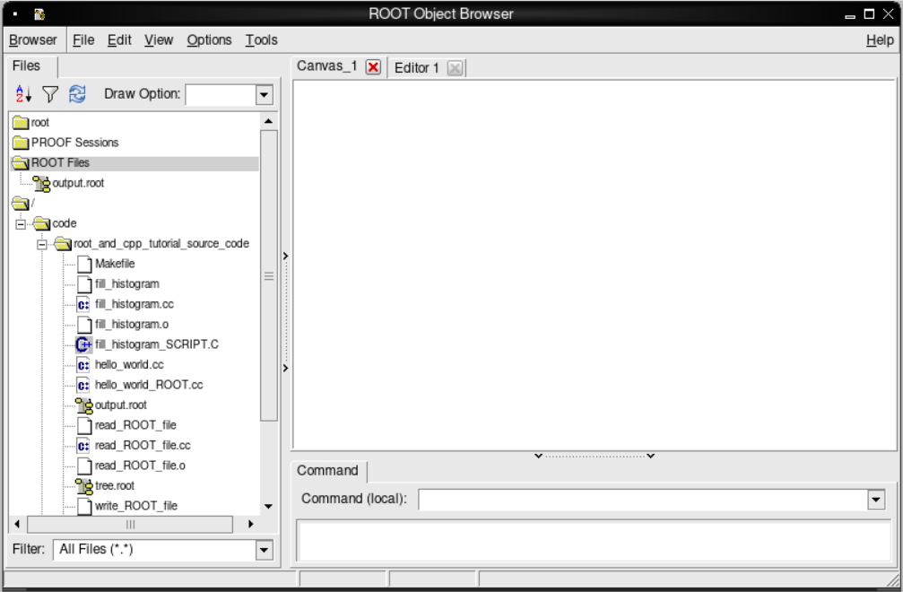
To inspect this new ROOT file, we’ll launch CINT for the first time
and create a TBrowser
object.
On the command line, run the following to launch CINT and attach our new ROOT file.
OUTPUT
root [0]
Attaching file output.root as _file0...
root [1]You can either type C++/ROOT commands or launch a
TBrowser, which is a graphical tool to inspect ROOT files.
Inside this CINT environment, type the following (without the
root [1], as that is just the ROOT/CINT prompt).
You should see the TBrowser pop up!
TBrowser
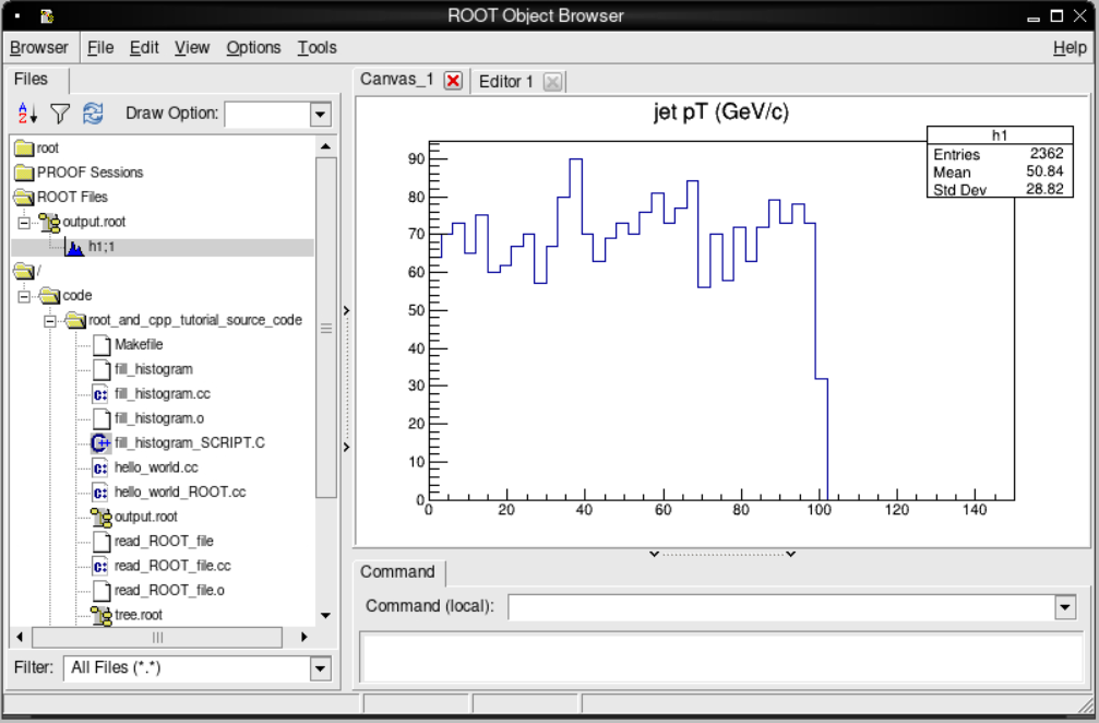
If we double click on output.root, in the left-hand menu
and then the h1;1 that appears below it, we should see the
following plot appear!
Inspecting the ROOT file contents
Quit ROOT by choosing the “Quit Root” option from Browser menu of the
TBrowser window or by typing .q in the ROOT prompt.
Work assignment: investigating data in ROOT files
In the previous episode you generated a file called
tree.root. It has some variables which were stored in a
TTree called t1. Let’s explore the variables contained in
this tree by using one of the methods available for TTree objects. You
can find out more about these methods directly from the ROOT TTree class
documentation.
Open the tree.root file with ROOT:
Now, dump the content of the t1 tree with the method
Print. Note that, by opening the file, the ROOT tree in
there is automatically loaded.
Please copy the output this statement generates and paste it into the corresponding section in our assignment form; remember you must sign in and click on the submit button in order to save your work. You can go back to edit the form at any time. Then, quit ROOT.
Using a ROOT script
We could also loop over all the events, create and save the
histogram, but also draw the histogram onto a TCanvas
object and have it pop up, all from a ROOT script and the CINT.
First, let’s copy over our C++ source code into a C++ script.
Next we’ll remove the headers at the beginning and even get rid of
the int main designation, though we keep the curly
brackets.
We’ll also define a TCanvas object on which we’ll plot
our histogram. After we do that, we “change directory” to the canvas and
draw our histogram. We can even save it to a .png file.
CPP
// Declare a TCanvas with the following arguments
// * Internal name of the TCanvas object
// * Title to be displayed when it is drawn
// * Width of the canvas
// * Height of the canvas
TCanvas *c1 = new TCanvas("c1", "Canvas on which to display our histogram", 800, 400);
c1->cd(0);
h1.Draw();
c1->SaveAs("h_pt.png");Your fill_histogram_SCRIPT.C should look like this:
CPP
{
// Here's the input file
// Without the 'recreate' argument, ROOT will assume this file exists to be read in.
TFile f("tree.root");
   // Let's make an output file which we'll use to save our
   // histogram
   TFile fout("output.root","recreate");
   // We define an histogram for the transverse momentum of the jets
   // The arguments are as follow
   // * Internal name of the histogram
   // * Title that will be used if the histogram is plotted
   // * Number of bins
   // * Low edge of the lowest bin
   // * High edge of the highest bin
   TH1F h1("h1","jet pT (GeV/c)",50,0,150);
// We will now "Get" the tree from the file and assign it to
// a new local variable.
TTree *input_tree = (TTree*)f.Get("t1");
Float_t met; // Missing energy in the transverse direction.
Int_t njets; // Necessary to keep track of the number of jets
// We'll define these assuming we will not write information for
// more than 16 jets. We'll have to check for this in the code otherwise
// it could crash!
Float_t pt[16];
Float_t eta[16];
Float_t phi[16];
// Assign these variables to specific branch addresses
input_tree->SetBranchAddress("met",&met);
input_tree->SetBranchAddress("njets",&njets);
input_tree->SetBranchAddress("pt",&pt);
input_tree->SetBranchAddress("eta",&eta);
input_tree->SetBranchAddress("phi",&phi);
// Get the number of events in the file
Int_t nevents = input_tree->GetEntries();
for (Int_t i=0;i<nevents;i++) {
// Get the values for the i`th event and fill all our local variables
// that were assigned to TBranches
input_tree->GetEntry(i);
// Print the number of jets in this event
printf("%d\n",njets);
// Print out the momentum for each jet in this event
for (Int_t j=0;j<njets;j++) {
printf("%f,%f,%f\n",pt[j], eta[j], phi[j]);
         // Fill the histogram with each value of pT
         h1.Fill(pt[j]);
}
}
// Declare a TCanvas with the following arguments
// * Internal name of the TCanvas object
// * Title to be displayed when it is drawn
// * Width of the canvas
// * Height of the canvas
TCanvas *c1 = new TCanvas("c1", "Canvas on which to display our histogram", 800, 400);
c1->cd(0);
h1.Draw();
c1->SaveAs("h_pt.png");
   fout.cd();
   h1.Write();
   fout.Close();
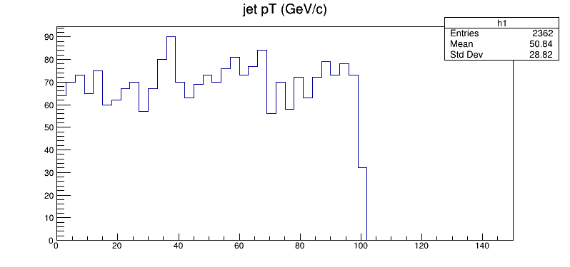
}To run this, you need only type the following on the command line.
You’ll be popped into the CINT environment and you should see the following plot pop up!
TBrowser
Exit from the container. If you are using a container with VNC, first
stop VNC with stop_vnc.
Key Points
- You can quickly inspect your data using just ROOT
- A simple ROOT script is often all you need for diagnostic work
Content from Using ROOT with python
Last updated on 2024-07-26 | Edit this page
Estimated time: 5 minutes
Overview
Questions
- Can I call ROOT from python?
Objectives
- Find resources for PyROOT
- Find resources for Scikit-HEP
PyROOT
The PyROOT project started with Wim Lavrijsen in the late `00s and became very popular, paralleling the rise of more general python tools within the community. Python has become the primary analysis language for the majority of HEP experimentalists. It has a rich ecosystem that is constantly evolving. This is a good thing because it means that improvements and new tools are always being developed, but it can sometimes be a challenge to keep up with the latest and greatest projects! :)
If you want to learn how to use PyROOT, you can go through some individual examples here, or a more guided tutorial here.
Feel free to challenge yourself to rewrite the previous C++ code using PyROOT!
Scikit-HEP libraries
Over the past several years, an effort has developed to provide more
python tools that can interface with CMS ROOT file formats as well as
typical scientific python tools used widely beyond particle physics. We
will use several of the Scikit-HEP
libraries to analyze NanoAOD: uproot, awkward,
and vector. As CMS datasets grow larger, we increasingly
rely on tools for array-based data processing in python, and the
scikit-HEP tools are very important for that task.
You can check out a tutorial for many of their tools here.
Using the Python docker container
The tools in the Python docker container will allow you to can easily open and analyze ROOT files. This is useful for when you make use of the CMS open data tools to skim some subset of the open data and then copy it to your local laptop, desktop, or perhaps an HPC cluster at your home institution.
If you completed the Docker pre-exercises you should already have worked through this episode, under Download the docker images for ROOT and python tools and start container, and you will have
- a working directory
cms_open_data_pythonon your local computer - a docker container with name
my_pythoncreated with the working directorycms_open_data_pythonmounted into the/codedirectory of the container.
Start your python container with
In the container, you will be in the /code directory and
it shares the files with your local cms_open_data_python
directory.
If you’re using apptainer:
Whenever you see a docker start instruction, replace it
with apptainer shell to open either the ROOT or Python
container image. The specific commands in this pre-exercise and during
the live workshop will be given for docker, since that is the most
common application. As a general rule, editing of files will be done in
the standard terminal (the containers do not have all text editors!) or
via the jupyter-lab interface, and then commands will be executed inside
the container shell. If you see Singularity> on your
command line, you are ready to run a ROOT or python script.
If you want to test out the installation, from within Docker you can
launch and interactive python session by typing python (in
Docker) and then trying
If you don’t get any errors then congratulations! You have a working environment and you are ready to perform some HEP analysis with your new python environment!
Key Points
- PyROOT is a complete interface to the ROOT libraries
- Scikit-HEP provides tools to interface between ROOT and global scientific python tools
- We will use
uproot,awkward, andvectorin our NanoAOD analysis
Content from Using uproot to open ROOT files
Last updated on 2024-07-09 | Edit this page
Estimated time: 20 minutes
Overview
Questions
- How do I open a ROOT file with uproot?
- How do I explore what is in the file?
Objectives
- Use a different library than ROOT to open ROOT files
- Get comfortable with a different way of examining ROOT files
Other resources
Before we go any further, we point out that this episode and the next
are only the most basic introductions to uproot
and awkward. There is a plethora of material that go much
deeper and we list just a few here.
How to type these commands?
Now that you’ve installed the necessary python modules in your
my_python container you can choose to write and execute the
code however you like. There are a number of options, but we will point
out two here.
-
Jupyter notebook. This provides an editor and an evironment in which to run your python code. Often you will run the code one cell at a time, but you could always put all your code in one cell if you prefer. There are many, many tutorials out there on using Jupyter notebooks and if you chose to use Jupyter as your editing/executing environment that you have developed some familiarity with it.
- In the
my_pythoncontainer, you can startjupyter-labwith
and open the link given in the message on your browser. Choose the icon under “Notebook”.
- In the
Python scripts. In this approach, you edit the equivalent of a text file and then pass that text file into a python interpreter. For example, if you edited a file called
hello_world.pysuch that it contained
You could save the file and then (perhaps in another Terminal window), execute
This would interpret your text file as python commands and produce the output
OUTPUT
Hello world!We leave it to you to decide which approach you prefer.
Open a file
Let’s open a ROOT file! If you’re writing a python script, let’s call
it open_root_file.py and if you’re using a Jupyter
notebook, let’s call it open_root_file.ipynb. If you are
working in the container, you will open and edit the python
script on your local computer and run it in the container, or
you will open a notebook on your jupyter-lab window in the browser.
First we will import the uproot library, as well as some
other standard libraries. These can be the first lines of your python
script or the first cell of your Jupyter notebook.
If this is a script, you may want to run
python open_root_file.py every few lines or so to see the
output. If this is a Jupyter notebook, you will want to put each snippet
of code in its own cell and execute them as you go to see the
output.
Let’s open the file! We’ll make use of uproots use of XRootD to read in the file
over the network. This will save us from having to download the
file.
PYTHON
infile_name = 'root://eospublic.cern.ch//eos/opendata/cms/derived-data/AOD2NanoAODOutreachTool/ForHiggsTo4Leptons/SMHiggsToZZTo4L.root'
infile = uproot.open(infile_name)Download the file?
If too many people are trying to open the same file, it may be easier to download the file to your laptop. You can execute the following command in the bash terminal.
PYTHON
curl http://opendata.cern.ch/record/12361/files/SMHiggsToZZTo4L.root --output SMHiggsToZZTo4L.rootAlternatively, you can follow this link to the data record on the CERN Open Data Portal. If you scroll down to the bottom of the page and click the Download button.
For the remainder of this tutorial you will want the file to be in the same directory/folder as your python code, whether you are using a Jupyter notebook or a simple python script. So make sure you move this file to that location after you have downloaded it.
To read in the file, you’ll change one line to define the input file to be
Investigate the file
So you’ve opened the file with uproot. What is this
infile object? Let’s add the following code
and we get
OUTPUT
<class 'uproot.reading.ReadOnlyDirectory'>We can interface with this object similar to how we would interface with a python dictionary.
OUTPUT
['Events;1']But what is this?
OUTPUT
<class 'uproot.models.TTree.Model_TTree_v20'>Ah, this is the TTree object that we learned a bit about
in the previous episodes! Let’s see what’s in it!
PYTHON
branches = infile['Events'].keys()
for branch in branches:
print(f"{branch:20s} {infile['Events'][branch]}")OUTPUT
run <TBranch 'run' at 0x7faa76d2cdd8>
luminosityBlock <TBranch 'luminosityBlock' at 0x7faa76d2cda0>
event <TBranch 'event' at 0x7faa76d13748>
PV_npvs <TBranch 'PV_npvs' at 0x7faa76d13e10>
PV_x <TBranch 'PV_x' at 0x7faa76d194e0>
PV_y <TBranch 'PV_y' at 0x7faa76d19ba8>
PV_z <TBranch 'PV_z' at 0x7faa76d212b0>
nMuon <TBranch 'nMuon' at 0x7faa76d21978>
Muon_pt <TBranch 'Muon_pt' at 0x7faa76d5c080>
Muon_eta <TBranch 'Muon_eta' at 0x7faa76d5c6d8>
Muon_phi <TBranch 'Muon_phi' at 0x7faa76d5ccc0>
Muon_mass <TBranch 'Muon_mass' at 0x7faa76d582e8>
Muon_charge <TBranch 'Muon_charge' at 0x7faa76d588d0>
Muon_pfRelIso03_all <TBranch 'Muon_pfRelIso03_all' at 0x7faa76d58eb8>
Muon_pfRelIso04_all <TBranch 'Muon_pfRelIso04_all' at 0x7faa76d4e4e0>
Muon_dxy <TBranch 'Muon_dxy' at 0x7faa76d4eac8>
Muon_dxyErr <TBranch 'Muon_dxyErr' at 0x7faa7443a0f0>
Muon_dz <TBranch 'Muon_dz' at 0x7faa7443a6d8>
Muon_dzErr <TBranch 'Muon_dzErr' at 0x7faa7443ad30>
nElectron <TBranch 'nElectron' at 0x7faa74442358>
Electron_pt <TBranch 'Electron_pt' at 0x7faa74442940>
Electron_eta <TBranch 'Electron_eta' at 0x7faa74442f28>
Electron_phi <TBranch 'Electron_phi' at 0x7faa7444a550>
Electron_mass <TBranch 'Electron_mass' at 0x7faa7444ab38>
Electron_charge <TBranch 'Electron_charge' at 0x7faa74451160>
Electron_pfRelIso03_all <TBranch 'Electron_pfRelIso03_all' at 0x7faa74451748>
Electron_dxy <TBranch 'Electron_dxy' at 0x7faa74451d30>
Electron_dxyErr <TBranch 'Electron_dxyErr' at 0x7faa74459358>
Electron_dz <TBranch 'Electron_dz' at 0x7faa74459940>
Electron_dzErr <TBranch 'Electron_dzErr' at 0x7faa74459f28>
MET_pt <TBranch 'MET_pt' at 0x7faa7445f550>
MET_phi <TBranch 'MET_phi' at 0x7faa7445fbe0>There are multiple syntax you can access each of these branches.
PYTHON
pt = infile['Events']['Muon_pt']
# or
pt = infile['Events/Muon_pt']
# or
pt = events.Muon_pt
# or
pt = events['Muon_pt']We’ll use that last one for this lesson just to save some typing. :)
In the next episode we’ll use the awkward array object
when we extract these data and see how we can use awkward
in a standard-but-slow way or in a clever-and-fast way!
Key Points
- You can use uproot to interface with ROOT files which is often easier than installing the full ROOT ecosystem.
Content from Using awkward arrays to analyze HEP data
Last updated on 2024-07-09 | Edit this page
Estimated time: 20 minutes
Overview
Questions
- What are awkward arrays?
- How do I work with awkward arrays?
Objectives
- Learn to use awkward arrays in a simple, naive way.
- Learn to use awkward arrays in a much faster way, making use of the built-in functionality of the library.
Why awkward?
A natural question to ask would be “Why do I have to learn about awkward? Why can’t I just use numpy?” And yes, those are two questions. :) The quick answers are: you don’t have to and you can! But let’s dig deeper.
Awkward-array is a newer python tool written by Jim Pivarski (Princeton) and others that allows for very fast manipulation of ``jagged” arrays, like we find in HEP. You definitely don’t have to use it, but we present it here because it can speed things up considerably…if you know how to write your code.
Similarly, you can of course use standard numpy arrays
for many parts of your analysis, but your data may not always fit into
numpy arrays without some careful attention to your code.
In either case, you’ll want to think about how to work with your data
once you get it out of your file.
Environment
Use the Python environment that you set up in the previous two lesson
pages, such as your my_python docker container. We leave it
up to you whether or not you write and execute this code in a script or
as a Jupyter notebook.
Numpy arrays: a review
Before we dive into awkward lets review some of the
awsome aspects of numpy arrays…and also examine their
limitations.
Let’s import numpy (if you have not already done that in
this python session).
Next, let’s make a simple numpy array to use for our
exmples.
OUTPUT
[1 2 3 4]Numpy arrays are great because we can perform mathematical operations on them and the operation is quickly and efficiently carried out on every member of the array.
PYTHON
y = 2*x
print(y)
print() # This just puts a blank line between our other print statements
z = x**2
print(z)
print()
a = np.sqrt(x)
print(a)OUTPUT
[2 4 6 8]
[ 1 4 9 16]
[1. 1.41421356 1.73205081 2. ]Note that in that last operation where we take the square root, we
made use of a numpy function sqrt. That
function
`knows" how to operate on the elements of a numpy array, as opposed to the standard pythonmathlibrary which does *not* know how to work withnumpy`
arrays.
So this seems great! However, numpy arrays break down
when you have arrays that are not 1D and cannot be expressed in a
regular
`n x m" format. For example, suppose you have two events and each event has two muons and you want to store the transverse momentum ($p_T$) for these muons in anumpy`
array.
OUTPUT
[[ 20.9 12.3]
[127.1 60.2]]
[[ 41.8 24.6]
[254.2 120.4]]Great! Everything looks good and we get our expected behavior!
Now, suppose there are 3 muons in the second event. Does this still work?
OUTPUT
[list([20.9, 12.3, 20.9, 12.3])
list([127.1, 60.2, 23.8, 127.1, 60.2, 23.8])]Wait…what??? It looks like it just duplicated the entries so now it
looks like we’re storing information for 4 muons in the first
event and 6 muons in the second event! A closer looks shows us
that while pt is a numpy array, the elements
are not arrays but python list objects, which behave
differently.
The reason this happened is that numpy arrays can’t deal
with this type of
`jagged" behavior where the first row of your data might have 2 elements and the second row might have 3 elements and the third row might have 0 elements and so on. For that, we needawkward-array`.
Access or download a ROOT file for use with this exercise
We’ll work with the same file as in the previous lesson. If you have jumped straight to this lesson, please go back and review how to access the file over the network or by downloading it.
Open the file
Stop!
If you haven’t already, make sure you have run through the previous lesson on working with uproot.
Let’s open this ROOT file! If you’re writing a python script, let’s
call it open_root_file_and_analyze_data.py and if you’re
using a Jupyter notebook, let’s call it
open_root_file_and_analyze_data.ipynb.
First we will import the uproot library, as well as some
other standard libraries. These can be the first lines of your python
script or the first cell of your Jupyter notebook.
If this is a script, you may want to run
python open_root_file_and_analyze_data.py every few lines
or so to see the output. If this is a Jupyter notebook, you will want to
put each snippet of code in its own cell and execute them as you go to
see the output.
PYTHON
import numpy as np
import matplotlib.pylab as plt
import time
import uproot
import awkward as akLet’s open the file and pull out some data.
PYTHON
# Depending on if you downloaded the file or not, you'll use either
infile_name = 'root://eospublic.cern.ch//eos/opendata/cms/derived-data/AOD2NanoAODOutreachTool/ForHiggsTo4Leptons/SMHiggsToZZTo4L.root'
# or
#infile_name = 'SMHiggsToZZTo4L.root'
# Uncomment the above line if you downloaded the file.

infile = uproot.open(infile_name)

events = infile['Events']

pt = events['Muon_pt']
eta = events['Muon_eta']
phi = events['Muon_phi']
Let’s inspect these objects a little closer. To access the actual
values, we’ll see we need to use the .array() member
function.
PYTHON
print(pt)
print()

print(pt.array())
print()

print(len(pt.array()))
print()

for i in range(5):
    print(pt.array()[i])
OUTPUT
<TBranch 'Muon_pt' at 0x7f01513a5c88>

[[63, 38.1, 4.05], [], [], [54.3, 23.5, ... 43.1], [4.32, 4.36, 5.63, 4.75], [], []]

299973

[63, 38.1, 4.05]
[]
[]
[54.3, 23.5, 52.9, 4.33, 5.35, 8.39, 3.49]
[]
Taking a closer look at the entries, we see different numbers of values in each ``row”, where the rows correspond to events recorded in the CMS detector.
So can we use manipulate this object like a numpy array? Yes! If we’re careful about accessing the array properly.
OUTPUT
[[126, 76.2, 8.1], [], [], [109, 47, 106, 8.66, 10.7, 16.8, 6.98], []]When we histogram, however, we need to make use of the
awkward.flatten function. This turns our
awkward array into a 1-dimensional array, so that we lose
all record of what muon belonged to which event.
PYTHON
print(ak.flatten(pt.array()))

plt.figure()
plt.hist(ak.flatten(pt.array()),bins=100,range=(0,100));
plt.xlabel(r'Muon $p_T$ (GeV/c)',fontsize=14)
OUTPUT
[63, 38.1, 4.05, 54.3, 23.5, 52.9, 4.33, ... 32.6, 43.1, 4.32, 4.36, 5.63, 4.75]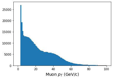
We can also manipulate the data quite quickly. Let’s see how!
This sample file is Monte Carlo data that simulates the decay of Higgs bosons to 4 charged leptons. Let’s look for decays to 4 muons, where there are two positively charged muons and 2 negatively charged muons.
Since the data stores momentum information as \(p_T, \eta, \phi\), first we’ll calculate the Cartesian \(x,y,z\) components of momentum, and then we’ll loop over our events to calculate an invariant mass. We’ll find that looping over the entries is slow, but there is a faster way!
First the slow but explicit way:
PYTHON
# Some helper functions

def energy(m, px, py, pz):
    E = np.sqrt( (m**2) + (px**2 + py**2 + pz**2))
    return E

def invmass(E, px, py, pz):
    m2 = (E**2) - (px**2 + py**2 + pz**2)

    if m2 < 0:
        m = -np.sqrt(-m2)
    else:
        m = np.sqrt(m2)
    return m

def convert(pt, eta, phi):
    px = pt * np.cos(phi)
    py = pt * np.sin(phi)
    pz = pt * np.sinh(eta)

    return px, py, pz

# Convert momentum to x,y,z components

muon_number = events['nMuon'].array()

pt = events['Muon_pt'].array()
eta = events['Muon_eta'].array()
phi = events['Muon_phi'].array()
muon_q = events['Muon_charge'].array()
mass = events['Muon_mass'].array()

muon_px,muon_py,muon_pz = convert(pt, eta, phi)
muon_e = energy(mass, muon_px, muon_py, muon_pz)

# Do the calculation

masses = []

nevents = len(pt)
print(f"Nevents: {nevents}")

start = time.time()

for n in range(nevents):

    if n%10000==0:
        print(n)

    nmuons = muon_number[n]

    e = muon_e[n]
    q = muon_q[n]
    px = muon_px[n]
    py = muon_py[n]
    pz = muon_pz[n]


    if nmuons < 4:
        continue

    for i in range(0, nmuons-3):
        for j in range(i+1, nmuons-2):
            for k in range(j+1, nmuons-1):
                for l in range(k+1, nmuons):

                    if q[i] + q[j] + q[k] + q[l] == 0:
                        etot = e[i] + e[j] + e[k] + e[l]
                        pxtot = px[i] + px[j] + px[k] + px[l]
                        pytot = py[i] + py[j] + py[k] + py[l]
                        pztot = pz[i] + pz[j] + pz[k] + pz[l]

                        m = invmass(etot, pxtot, pytot, pztot)
                        masses.append(m)

print(f"Time to run: {(time.time() - start)} seconds")

# Plot the results

plt.figure()
plt.hist(masses,bins=140,range=(80,150))
plt.xlabel(r'4-muon invariant mass (GeV/c$^2$',fontsize=18)
plt.show()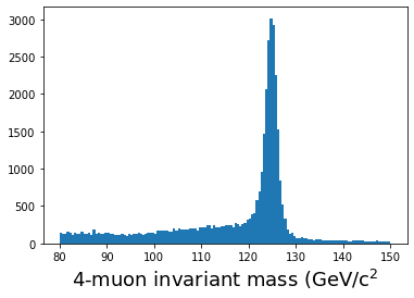
When I run this on my laptop, it takes a little over 3 minutes to run. Is there a better way?
Yes!
We’ve adapted some code from this tutorial, put together by the HEP Software Foundation to show you how much faster using the built-in awkward functions can be:
PYTHON
start = time.time()

muons = ak.zip({
    "px": muon_px,
    "py": muon_py,
    "pz": muon_pz,
    "e": muon_e,
    "q": muon_q,
})

quads = ak.combinations(muons, 4)

mu1, mu2, mu3, mu4 = ak.unzip(quads)

mass_fast = (mu1.e + mu2.e + mu3.e + mu4.e)**2 - ((mu1.px + mu2.px + mu3.px + mu4.px)**2 + (mu1.py + mu2.py + mu3.py + mu4.py)**2 + (mu1.pz + mu2.pz + mu3.pz + mu4.pz)**2)

mass_fast = np.sqrt(mass_fast)

qtot = mu1.q + mu2.q + mu3.q + mu4.q

print(f"Time to run: {(time.time() - start)} seconds")

plt.hist(ak.flatten(mass_fast[qtot==0]), bins=140,range=(80,150));
plt.xlabel(r'4-muon invariant mass (GeV/c$^2$',fontsize=18)
plt.show()
On my laptop, this takes less than 0.2 seconds! Note that we are
making use of boolean
arrays to perform masking when we type
mass_fast[qtot==0].
While we cannot teach you everything about
awkward, we hope we’ve given you a basic introduction to
what it can do and where you can find more information so that you can
quickly process the output of any of your open data jobs and get started
on your own analysis!
Key Points
- Awkward arrays can help speed up your code, but it requires a different way of thinking and more awareness of what functions are coded up in the awkward library.