Intro Reading
Overview
Teaching: 30 min
Exercises: 0 minQuestions
Did you do the pre-learning module?
Objectives
Review the treatment of jets in CMS before the Advanced Physics Objects lesson
To prepare for this lesson, please follow or review the Physics Objects Pre-learning modules on jets, b-tagging, and jet energy corrections.
Key Points
Join us in tomorrow’s sessions for the rest of the lesson.
Intro to Particle Flow
Overview
Teaching: 30 min
Exercises: 10 minQuestions
What is the CMS Particle Flow algorithm?
How are particle candidates classified with Particle Flow?
How can Particle Flow information be accessed in POET?
Objectives
Understand the 5 types of particle flow candidates
Investigate particle flow candidates in POET
Particle Flow in CMS
“The CMS particle-flow algorithm aims to identify and reconstruct individually all of the particles produced in a collision, through an optimal combination of the information from the entire detector. These particles are then used to build higher-level physics objects, such as jets, and the missing transverse momentum, with superior resolution.”
The concept of “particle flow” began at LEP, and has been used consistently by CMS. This method maps the mental picture of a particle “flowing” through multiple subdetectors onto the reconstruction method. Particle flow allows the resolution of tracking detectors and electromagnetic calorimeters to supplement information from hadronic calorimeters when reconstructing jets, missing transverse energy, tau leptons, and estimating pileup contributions.
The PF algorithm takes in tracks from the inner tracker, ECAL energy deposits, HCAL energy deposits, and muon chamber tracks. First, the calorimeter energy deposits are connected into clusters, and then all of the tracks and clusters are linked to each other based on spatial proximity. Blocks can be formed from groups of linked tracks and clusters, and from these blocks particle candidates can be separated out. The resulting list of “particle flow candidates” becomes the input to any event interpretation algorithms in CMS, such as jet clustering.
Clustering
Clustering proceeds in three basic steps:
- Identify topological clusters: a topological cluster is a group of calorimeter cells, each registering an energy deposit above a certain threshold, that share at least one neighbor.
- Identify seeds: a “seed” is any calorimeter cell whose energy is a local maximum, with respect to its immediate neighbors. Topological clusters must have 1 seed, but may have multiple.
- Compute cluster positions and energies: easier said than done!
- Single-seed topological clusters: the cluster energy is the sum of all the individual cell energies within the topological cluster, and the cluster position is found from the energy-weighted average of the individual cell positions.
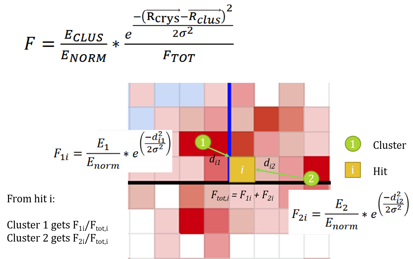
- Multiple-seed topological clusters: each seed is assumed to represent a unique energy cluster, but the energy deposited in non-seed cells must be shared between the various clusters within the topological cluster. An iterative procedure is used to converge on cluster energies and positions based on energy-weighted averages of fractional cell energies. The images below show an example of this type of cluster, with cells represented as squares in \(\eta-\phi\) space.

Links and Blocks
Linking is the procedure of connecting together tracks and clusters based on their spatial proximity. This is almost simpler to do “by eye” than computationally! In practice, a web of links is created between tracks and clusters, something like a dense neural network map, and only the “shortest” links are kept. In simplified language, the following “rules” show which links would be kept in particle flow:
Linking Rules
Connect a small thing to one big thing They must be “touching” in \(\eta-\phi\) space! (+1 cell buffer zone is ok too) The closest big thing wins the link!
Links can be formed between tracks and ECAL clusters, tracks and HCAL clusters, ECAL clusters and HCAL clusters, inner tracks and muon tracks, muon tracks and ECAL clusters, and muon tracks and HCAL clusters. After all the links are established, “blocks” are formed from all groups of linked tracks and clusters:
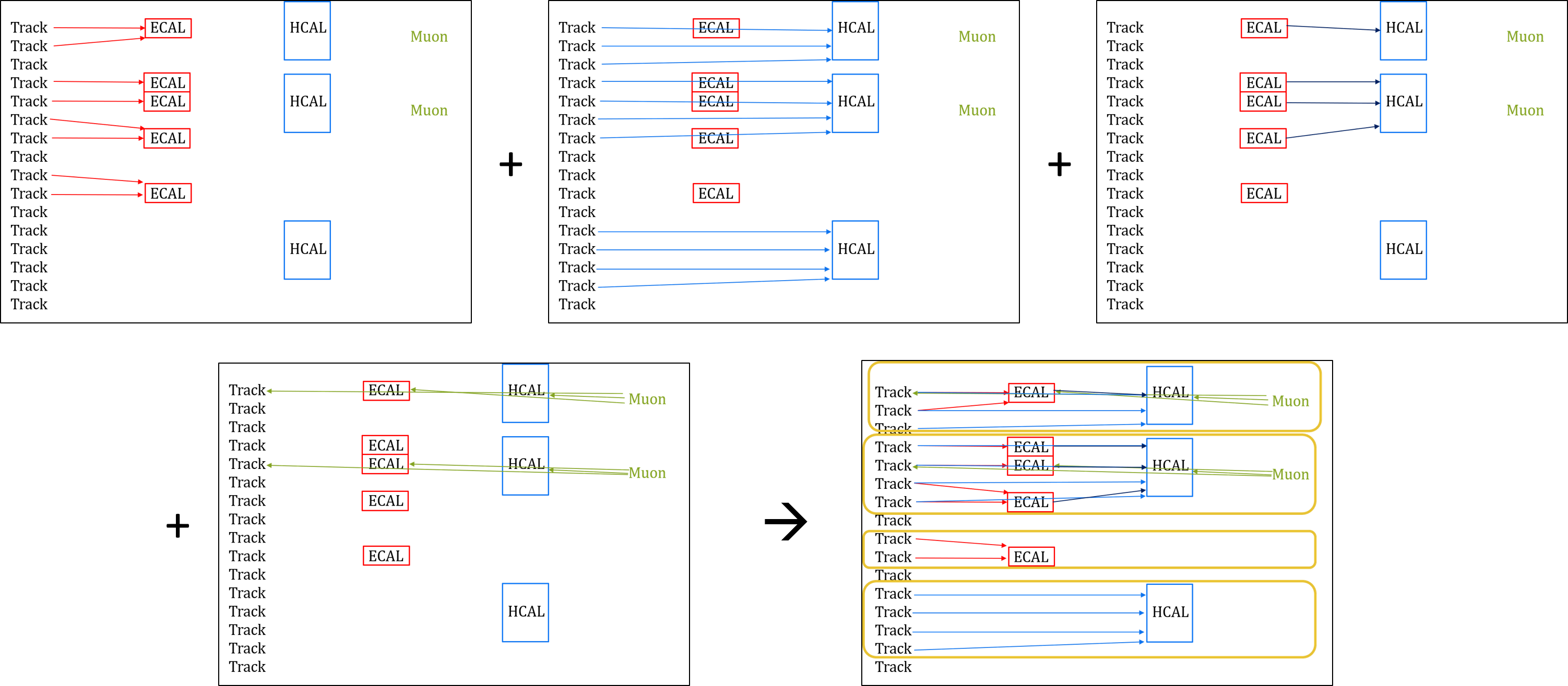
Blocks are also constructed from any “lone” elements, such as single tracks or single clusters.
Candidate formation
Next, blocks are redivided into particle candidates, following a strict order of decision making. After checking, in order, for each type of particle listed below, the tracks/clusters associated with each newly formed candidate are removed from their blocks.
Muons
Inner tracks linked to muon tracks are called “Global Muons”. If there is little calorimeter energy nearby, all linked ECAL and HCAL clusters are assigned to the muon. In regions with significant calorimeter activity, clusters linked directly to the muon tracks as assigned to the muon if it passes the “tight” identification working point.
Muon momentum and direction
- Inner track momentum and angles are assigned for muon with pT < 200 GeV
- Very high pT muons need more care (FIXME)
Isolated electrons and photons
ECAL clusters that are not linked to HCAL clusters are considered isolated electrons or photons. A photon candidate is formed if there are no track links and the ECAL cluster has at least 10 GeV of energy. An electron candidate is formed if a 2+ GeV track is linked to the ECAL cluster, and its momentum is very similar to the ECAL cluster’s energy. The algorithm accounts for bremsstrahlung radiation and pair production within the tracker when assigning block elements to electrons.
Electron and photon momentum and direcion
- Photons: calibrate the ECAL cluster’s energy, and assign the cluster’s energy and direction to the photon.
- Electrons: calibrate the ECAL cluster’s energy and assign that energy to the electron, but assign the track’s direction.
Neutral hadrons and photons
Next particle flow considers all other clusters without track links. Any such ECAL cluster is assigned as a photon candidate, and any such HCAL cluster is assigned as a neutral hadron candidate.
Neutral candidate energy and direction
Calibrate the ECAL or HCAL energy and assign the cluster’s energy and direction to the photon or neutral hadron.
Charged hadrons
Everything that’s left are charged hadrons!
At this point, all the tracks and clusters related to muons, electrons, photons, and neutral hadrons have been removed from the PF blocks. The remaining question is how many charged hadrons to assign in each block, and what their properties should be. First, the energy must be calibrated: the sum of cluster energy is compared to the sum of track momenta and the larger of those two values is used to calibrate the energy of the cluster group. Then, 3 cases can be considered:
-
The track momentum sum is smaller than the calibrated cluster energy sum. In this case, each track is assigned as a charged hadron candidate carrying the track’s momentum and direction. The excess energy (calculated assuming the tracks represent charged pions) from clusters links to each track is assigned as photon candidates and neutral hadron candidates, depending on the type of clusters that are found.
-
The track momentum sum agrees with the calibrated cluster energy sum, within the energy resolution. In this case, each track is assigned as a charged hadron candidate carrying the track’s momentum and direction.
-
The track momentum sum is larger than the calibrated cluster energy sum. This indicates that either a muon or a track has been significantly mismeasured! The algorithm walks through several checks of track uncertainties and other features to try and remedy the error.
The final step in candidate formation is to assign “lone” tracks as charged hadrons carrying the track’s momentum and direction.
Charged hadron energy and direction
Typically, charged hadrons are assigned the momentum and direction of their linked track, assuming the pion mass. Excess cluster energy can be assigned as photons and/or neutron hadrons, using the calibrated cluster energy and direction.
Event interpretation
The particle flow candidates can now be fed into any event-wide algorithm you list: jet clustering, MET calculations, hadronic tau reconstruction, pileup mitigation techniques, neural network jet taggers, and many more. If you would like to learn more about this topic, the Particle Flow paper is a great read!
POET particle flow candidates
In MiniAOD files, the particle flow candidates are accessible through the packedPFCandidates collection. Particle flow is run in the “RECO” step of CMS data processing, but specific information about the candidates are kept in AOD and MiniAOD files. A summary of the information available in MiniAOD files can be found on the 2015 MiniAOD Workbook TWiki.
The PackedCandidateAnalyzer is configured in poet_cfg.py to access this collection:
process.mypackedcandidate = cms.EDAnalyzer('PackedCandidateAnalyzer',
                                           packed=cms.InputTag("packedPFCandidates")
                                           )
The analyzer itself is simple, pulling out kinematic and labelling information for each candidate. More methods exist and are documented in the PAT::PackedCandidate class.
   for (const pat::PackedCandidate &pack : *packed)
   {
         packed_pt.push_back(pack.pt());
         packed_eta.push_back(pack.eta());
         packed_mass.push_back(pack.mass());
         packed_energy.push_back(pack.energy());
         packed_phi.push_back(pack.phi());
         packed_ch.push_back(pack.charge());
         packed_px.push_back(pack.px());
         packed_py.push_back(pack.py());
         packed_pz.push_back(pack.pz());
         packed_theta.push_back(pack.theta());
         packed_vx.push_back(pack.vx());
         packed_vy.push_back(pack.vy());
         packed_vz.push_back(pack.vz());
         packed_lostInnerHits.push_back(pack.lostInnerHits());
         packed_PuppiWeight.push_back(pack.puppiWeight());
         packed_PuppiWeightNoLep.push_back(pack.puppiWeightNoLep());
         packed_hcalFraction.push_back(pack.hcalFraction());
         packed_pdgId.push_back(pack.pdgId());
       numCandidates++;
    }
What are PF Candidate PDG IDs?
- 11, 13 = electron, muon
- 22 = photon
- 130 = neutral hadron
- 211 = charged hadron
- 1 = hadronic particle reconstructed in the forward calorimeters
- 2 = electromagnetic particle reconstructed in the forward calorimeters
Run POET with PF candidates included
We will need to uncomment the PF candidate analyzer in the path at the bottom of
poet_cfg.py. Your path for MC should look like this:else: process.p = cms.Path(process.hltHighLevel+process.elemufilter+process.mysimpletrig+ process.myelectrons+process.mymuons+process.mytaus+process.myphotons+process.mypvertex+process.mygenparticle+ process.looseAK4Jets+process.patJetCorrFactorsReapplyJEC+process.slimmedJetsNewJEC+process.myjets+ process.looseAK8Jets+process.patJetCorrFactorsReapplyJECAK8+process.slimmedJetsAK8NewJEC+process.myfatjets+ process.uncorrectedMet+process.uncorrectedPatMet+process.Type1CorrForNewJEC+process.slimmedMETsNewJEC+process.mymets +process.mypackedcandidate )Run poet over 100 MC events (set
maxEventsback to 100!)cmsRun python/poet_cfg.py TrueOpen
myoutput.rootand try to plot the PF candidate PDG ID – how do the abundances vary? It is also interesting to compare the sizemyoutput.rootwith and without including the PF candidates – we do not include them by default since they can increase the file size by a significant amount!
Key Points
Particle Flow connects information from all CMS subdetectors to form particle trajectories.
Particle Flow candidates are labelled as muons, electrons, photons, charged hadrons, and neutral hadrons.
When enabled, POET files can contain 4-vector and labelling information for all of the particle flow candidates.
Jet substructure
Overview
Teaching: 15 min
Exercises: 25 minQuestions
Which jet substructure observables are available in CMS MiniAOD?
How are W boson jets identified using fat jets?
How are top quark jets identified using fat jets?
Objectives
Understand the groomed mass and jet substructure variables typically used in CMS analyses
Study W boson and top quark identification
Download a POET output file
In the pre-learning lesson you may have processed a full high-mass \(t\bar{t}\) file through POET. A copy of the output can be accessed here. You can pull it into your CMSSW or ROOT docker container:
wget https://jmhogan.web.cern.ch/jmhogan/OpenData/myoutput_ttbarM1000.rootFor the following lesson you can interact with this file in either the CMSSW or ROOT docker containers.
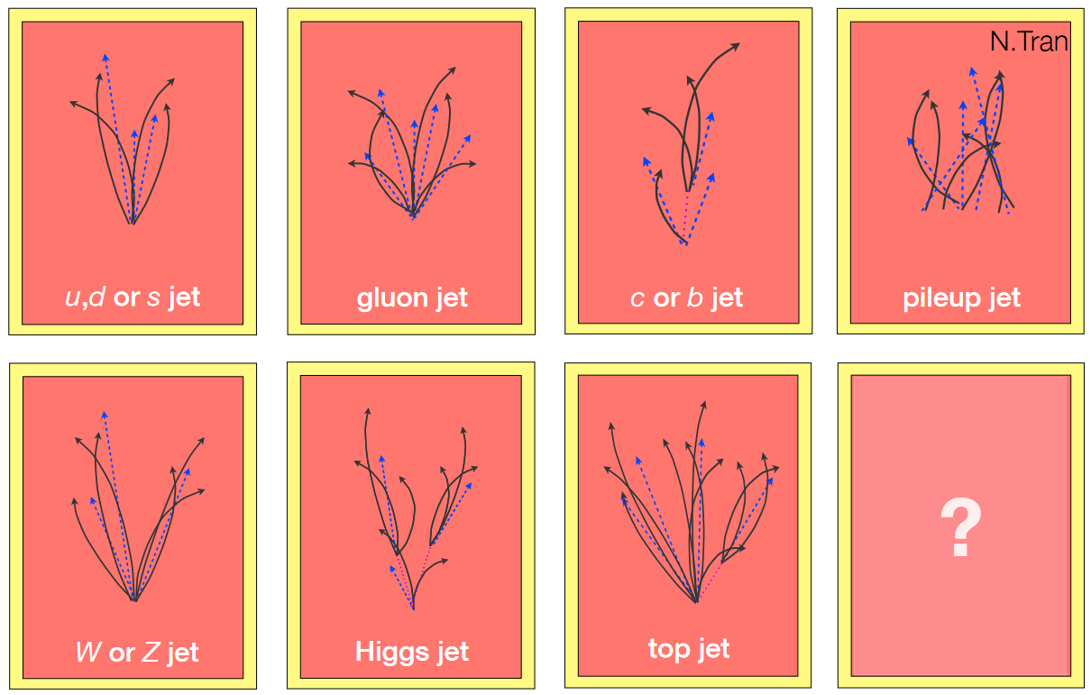
Jets can originate from many different types of particles. The figure below gives an example of how different “parent particles” can influence the internal structure of a jet. Observables related to the mass and internal structure of a jet can help us design algorithms to distinguish between sources. The most common type of algorithm identifies b quark jets from light quark or gluon jets. The POET contains all the tools you need to evaluate the default CMS b tagging discriminants on small-radius jets. See the next episode for more information. In this lesson we will focus on tools to identify hadronic decays of Lorentz-boosed massive SM particles within large-radius jets.

Jet mass and grooming
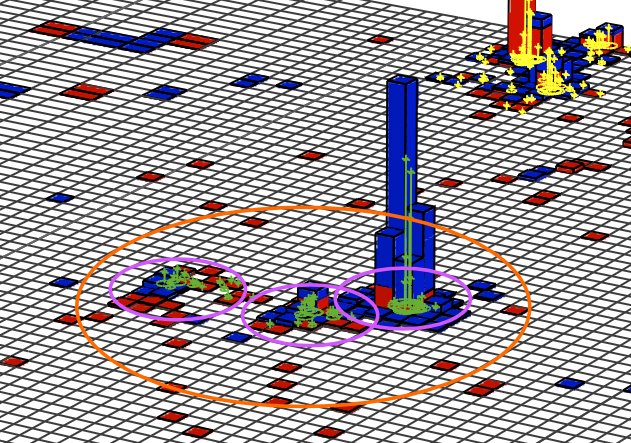
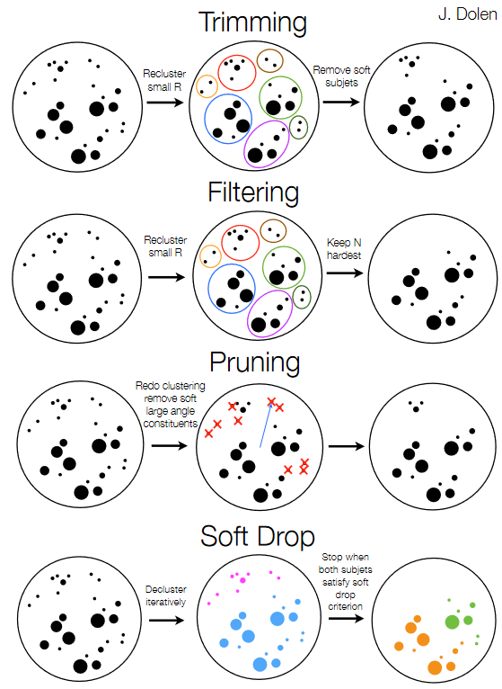
The mass of a jet is evaluated by summing the energy-momentum four-vectors of all the particle flow candidates that make up the jet and computing the mass of the resulting object. This mass calculation is distorted by the low-momentum and wide-angle gluon radiation emerging from the initial hadrons that formed the jet. For example, the masses of light quark or gluon jets are measured to be much larger than the actual masses of these particles – typically 10–50 GeV with a smooth continuum to higher values. Grooming procedures can help reduce the impact of this radiation and bring the jet mass closer to the true values of the parent particles. Grooming algorithms typically cluster the jet’s consitituents into “subjets”, like those represented by the small circles in the figure below. The relationships between different subjets can then be tested to decide which to keep.

Four groomed masses are available for large-radius (“fat”) jets in 2015 MiniAOD:
- Trimmed mass: jets are reclustered using a small distance parameter, and any “subjets” that have too small a fraction of the original jet momentum are discarded.
- Filtered mass: jets are reclustered using a small distance parameter, and a certain number of subjets are kept.
- Pruned mass (default for identifying W/Z/H boson jets): jets are reclustered, and at each step subjets that are too soft or at large angles are discarded.
- Soft drop mass (default for identifying t quark jets): jets are recursively de-clustered, and at each step jets that are too soft or at large angles are discarded.

In FatjetAnalyzer.cc the groomed masses are accessed via the “userFloat” method available in all PAT classes. This implies that a value has been calculated elsewhere and the result stored manually inside the PAT object. In the case of jet masses, it is important to note that userFloat values are not automatically corrected when “jet energy corrections” are applied. These corrections are covered in the last segment of this lesson – in POET specific levels of correction are applied to the groomed masses.
fatjet_prunedmass.push_back(corrL2L3*(double)smearedFatjet.userFloat("ak8PFJetsCHSPrunedMass"));
fatjet_softdropmass.push_back(corrL2L3*(double)smearedFatjet.userFloat("ak8PFJetsCHSSoftDropMass"));
Exercise: boosted particle momentum ranges
Study the connection between jet mass and jet momentum – what minimum transverse momentum is required for W boson and top quark jets to be found within a large-radius jet?
Begin by opening the
myoutput_ttbarM1000.rootfile you processed at the beginning of this segment. Use ROOT’s capability to draw two-dimensional histograms to compare various jet masses against the jet’s transverse momentum:$ root -l myoutput_ttbarM1000.root [1] _file0->cd("myfatjets"); [2] Events->Draw("fatjet_<SOME MASS VARIABLE>:fatjet_corrpt","","colz"); // colz makes a heatmapSolution
This plot shows the relationship between momentum, mass, and jet radius. As the momentum increases, jets of larger mass become contained within the fat jet. While W bosons can be observed from 200 GeV, top quarks require a higher momentum threshold.
Jet substructure
The internal structure of a jet can be probed using many observables: N-subjettiness, energy correlation functions, and others. In CMS, N-subjettiness is the default jet substructure variable for identifying boosted particle decays.
The “tau” variables of N-subjettiness, defined below, are jet shape variables whose value approaches 0 for jets having N or fewer subjets:

If the value approaches zero it indicates that the consitituents all lie near one of the previously identified subjet axes. For a top quark jet with 3 subjets, we would expect small tau values for N = 3, 4, 5, 6, etc, but larger values for N = 1 or 2.
Ratios of tau values provide the best discrimination for jets with a specific number of subjets. For two-prong jets like W, Z, or H boson decays, we study the ratio tau_2 / tau_1. For three-prong jets we study tau_3 / tau_2.
In FatjetAnalyzer.cc, the N-subjettiness values are also accessed from userFloats:
fatjet_tau1.push_back((double)smearedFatjet.userFloat("NjettinessAK8:tau1"));
fatjet_tau2.push_back((double)smearedFatjet.userFloat("NjettinessAK8:tau2"));
fatjet_tau3.push_back((double)smearedFatjet.userFloat("NjettinessAK8:tau3"));
For top quark or H boson decays, applying b tagging algorithms to the subjets of the large-radius jets gives another valuable substructure observable. The Combined Secondary Vertex v2 discriminant, described in detail in the next episode, has been stored for the two subjets obtained from the soft drop algorithm in each large-radius jet. For simulation, we also store the generator-level flavor information for the subjet.
auto const & sdSubjets = smearedFatjet.subjets("SoftDrop");
int nSDSubJets = sdSubjets.size();
if(nSDSubJets > 0){
    pat::Jet subjet1 = sdSubjets.at(0);
    fatjet_subjet1btag.push_back(subjet1.bDiscriminator("pfCombinedInclusiveSecondaryVertexV2BJetTags"));
    fatjet_subjet1hflav.push_back(subjet1.hadronFlavour());
}else{
    fatjet_subjet1btag.push_back(-999);
    fatjet_subjet1hflav.push_back(-999);
}
// then the same for the 2nd subjet
Exercise: mass and N-subjettiness correlations
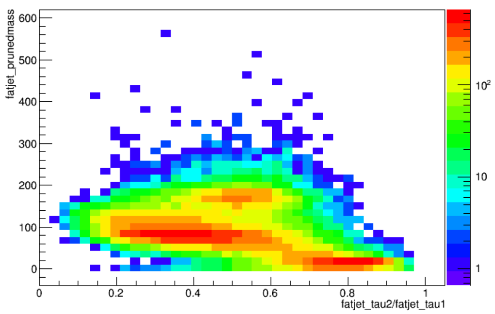
Study the correlation between groomed jet mass and N-subjettiness ratios. Make 2D plots of either pruned jet mass versus tau_2/tau_1, or softdrop jet mass versus tau_3/tau_2. Where do the various parent particles of the jets pool? What requirements would effectively select W bosons or top quarks? Tip: use the same type of ROOT Draw command as in the previous exercise.
Solution
The structure in the tau_2/tau_1 plot is very unique: W bosons pool at lower values of tau_2/tau_1, while top quarks (with more than 2 subjets) and light quarks (with only 1 subjet) pool at medium and higher values. In the tau_3/tau_2 plot, top quark jets have low values while both W boson and light quark jets are gathered near 1. The correlations in these plots lead directly to the “tagging” criteria introduced in the next section.

W and top tagging
The CMS jet algorithms group studied the efficiency of identifying known W boson jets using almost 30 different combinations of groomed mass and jet substructure variables. The optimal combination for 2015 data was pruned mass + tau_2/tau_1 for large-radius jets using the CHS pileup mitigation technique. For “PUPPI” jets, developed for Run 2, the softdrop mass is used instead. The use of PUPPI jets became the default for CMS analyses beginning only in 2016, so currently this option is not implemented in the POET.
Selection criteria for W boson and top quark jets in 2015 data analyses are described in this Physics Analysis Summary, including the calculations of corrections factors for simulation.
W boson selections
A W jet has pruned mass between 65 – 105 GeV and tau_2/tau_1 less than a chosen upper bound. The supported working points and their correction factors are shown in this table:


For top quarks, the soft drop mass is used regardless of pileup mitigation technique for the jets. In this case, tau_3/tau_2 becomes the most useful substructure variable, followed by b quark tagging applied on the individual subjets of the large-radius jet.
Top quark selections
A top quark jet has soft drop mass between 105 – 220 GeV, tau_3/tau_2 less than a chosen upper bound, and possibly a requirement on a subjet b quark tag. The supported working points, their efficiencies, and correction factors are shown in this table:


Exercise: explore jet tagging criteria
Study the connection between groomed mass, n-subjettiness ratios, and subjet b-tagging. From the top quark events in
myoutput_ttbarM1000.root, can you see either a W boson or top quark mass peak become visible in thefatjet_prunedmassorfatjet_softdropmassdistribution as you apply the various substructure criteria?Recall:
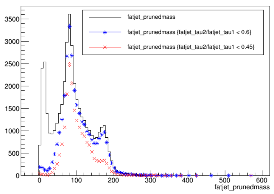
Events->Draw("fatjet_X","fatjet_Y > VALUE")will draw the branchfatjet_Xfor all events in whichfatjet_Y > VALUE. Adding a third parameter to the Draw command that says “same” will place a new histogram on top of any existing histograms.Criteria you could test include:
fatjet_tau2/fatjet_tau1 < 0.6fatjet_tau2/fatjet_tau1 < 0.45fatjet_corrpt > 500fatjet_tau3/fatjet_tau2 < 0.81fatjet_tau3/fatjet_tau2 < 0.57fatjet_subjet1btag > .046Solution
Both the W boson jets and the top quark jets can be isolated from the other jet types quite effectively with the N-subjettiness criteria!

Key Points
Grooming algorithms remove soft and wide angle radiation to bring a jet’s mass closer to that of the parent particle.
Substructure algorithms provide information about the number of high-momentum subjets or whether heavy flavor hadrons existed inside the jet.
The standard variables needed to tag W, Z, H boson or top quark jets in 2015 data are included in the POET.