Introduction
Overview
Teaching: 15 min
Exercises: 0 minQuestions
What is ADL?
What is CutLang?
Why would we use ADL/CutLang to write and perform analyses?
Objectives
Understand the concept of ADL and its main principles.
Understand the distinction between using ADL and using a general purpose language for writing analyses.
Understand the concept of runtime interpreter.
What is ADL?
(More information on cern.ch/adl)
LHC data analyses are usually performed using complex analysis frameworks written in general purpose languages like C++ and, more recently, Python. This method is very flexible, and usually is easy for simple analyses with simple selections. But what if we had a really complex analysis with very complex object and event selections. For example, take a look at the graph below, which describes a CMS search for supersymmetry (arXiv:2205.09597):
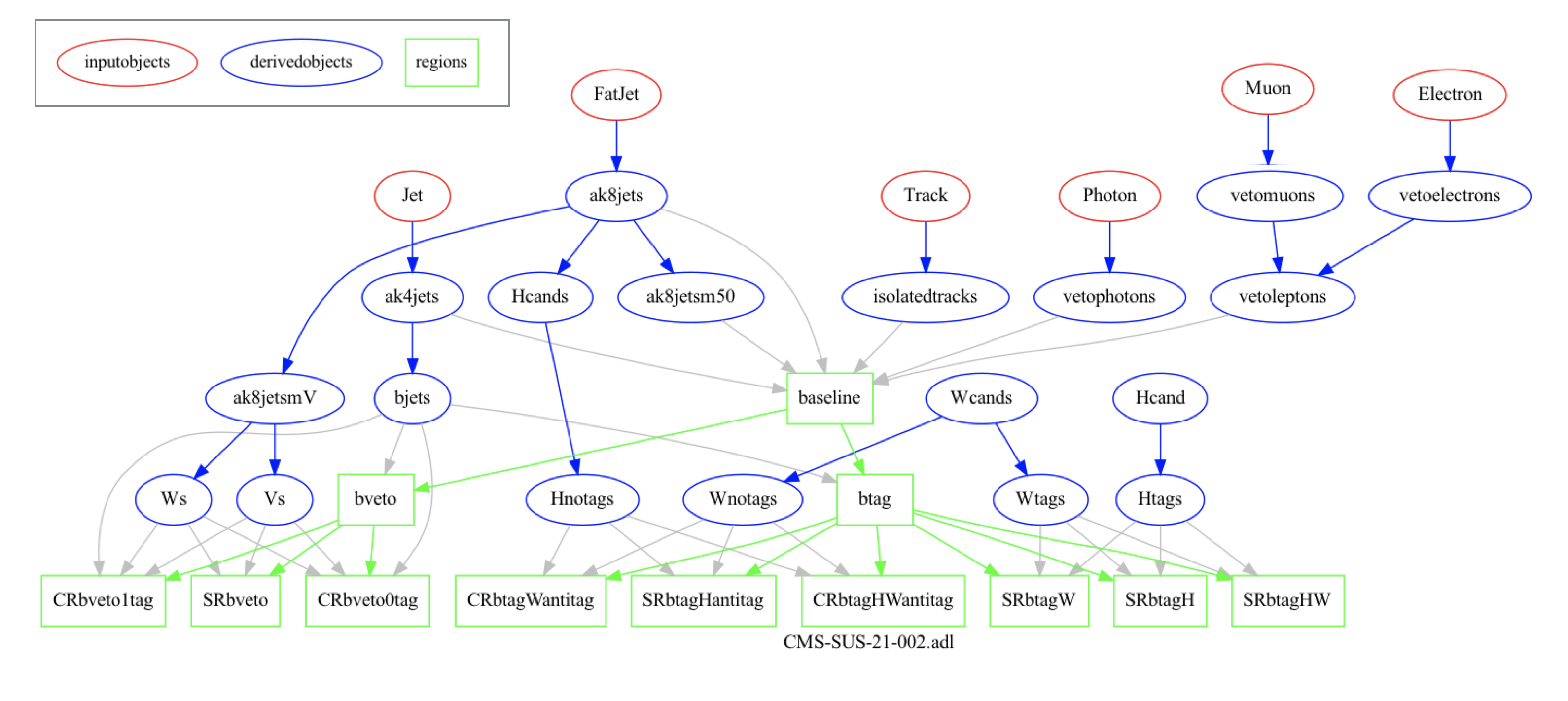
This analysis works with several different types of objects and multiple event selection regions, some of which are dependent on each other. When we write such an analysis with a general purpose language, it becomes increasingly harder to visualize and keep track of the physics algorithm details. As the analysis physics content becomes more intricate, analysis code will become more complex, and harder to follow.
The main reason behind this is that, when we write code using general purpose languages, we intertwine the physics algorithm with other technical details, e.g. accessing files, accessing variables, importing modules, etc. Despite the flexibility, all such technicalities obscure the code.
However there is another emerging alternative which allows to decouple physics algorithm from the technical code and write analyses with a simple, self-describing syntax. Analysis Description Language (ADL) is a HEP-specific analysis language developed with this purpose. Its main aim is to describe analyses in a more intuitive and physics-focused way.
More formally, ADL is a declarative domain specific language (DSL) that describes the physics content of a HEP analysis in a standard and unambiguous way.
- External DSL: Custom-designed syntax to express analysis-specific concepts. Reflects conceptual reasoning of particle physicists. Focus on physics, not on programming.
- Declarative: Tells what to do, but not how to do it.
- Human readable: Clear, self-describing syntax rules.
- Designed for everyone: experimentalists, phenomenologists, students, interested public…
ADL is designed to be framework-independent. Any framework recognizing ADL can perform tasks with it. Physics information becomes independent from software and framework details. This allows:
- Multi-purpose use of analysis description: Can be automatically translated or incorporated into the GPL / framework most suitable for a given purpose, e.g. exp, analysis, (re)interpretation, analysis queries, …
- Efficient communication between groups: experimentalists, phenomenologists, referees, students, public, …
- Accessible preservation of analysis physics logic.
ADL mainly focuses on describing event processing. This includes object selections, event variable definitions and event selections. It can also described histogramming, and partially systematic uncertainties.
ADL consists of blocks separating object, variable and event selection definitions for a clear separation of analysis components. Blocks have a keyword-expression structure. Keywords specify analysis concepts and operations. Syntax includes mathematical and logical operations, comparison and optimization operators, reducers, 4-vector algebra and HEP-specific functions (dphi, dR, etc.).
ADL is designed with the goal to be self-describing, so especially for simple cases, one does not need to read syntax rules to understand an ADL description. However if you are interested, the set of syntax rules can be found here.
ADL is a standard, which allows all analyses to be described in the same way. Having access to many analyses written in the same way can help us understand them easier, learn their physics logic easily, and use them in our own studies.
What is CutLang?
Once an analysis is written it needs to be run on events. This is achieved by CutLang , the runtime interpreter that reads and understands the ADL syntax and runs it on events. A runtime interpreter does not require to be compiled. The user only modifies the ADL description, and runs CutLang. CutLang is also a framework which automatically handles many tedious tasks as reading input events, writing output histograms, etc. CutLang can be run on various environments such as linux, mac, conda, docker, jupyter, etc.
In case you are interested to learn more on CutLang, please see the CutLang github and references in the cern.ch/adl) portal.
Key Points
ADL is a declarative domain specific language (DSL) that describes the physics content of a HEP analysis in a standard and unambiguous way.
ADL’s purpose is to decouple the physics logic of analyses from technical operations, and make the physics logic more accessible.
CutLang is a runtime interpreter that reads and understands the ADL syntax and runs it on events.
Installing CutLang
Overview
Teaching: 0 min
Exercises: 20 minQuestions
How do I access information about CutLang in general?
How do I install CutLang via Docker?
How do I test my installation?
Objectives
Setup CutLang via Docker
Understand the most basic concepts about running CutLang
Perform a test run with CutLang on an open data POET ntuple and check the output
Please make sure that you prepare the CutLang setup before the exercise.
Installing CutLang: introduction
CutLang is the runtime interpreter we will use for processing ADL files on events.
CutLang is compatible multiple platforms. It can be installed directly on Linux and MacOS, on all platforms via Docker or Conda, or can be accessed via a Jupyter/Binder interface.
The generic and most up-to-date instructions for setting up CutLang can be found in the CutLang github readme
In this exercise, we will use run CutLang via a docker container as described in the next section.
CutLang setup via Docker
We have prepared a CutLang docker container which functions similarly to other Docker containers that work with CMS Open Data. The setup contains:
- CutLang
- ROOT
- xrootd access to open data ntuples
- VNC
- Jupyter
- As a first step, make sure that you have Docker desktop installed.
You can find detailed instructions on how to install Docker and on simple Docker concepts and commands in this tutorial.
- Next, download the CutLang image and run container in current directory from downloaded image
For linux/MacOS:
docker run -p 8888:8888 -p 5901:5901 -p 6080:6080 -d -v $PWD/:/src --name CutLang-root-vnc cutlang/cutlang-root-vnc:latest
If you would like to re-run by mounting another directory, you should stop the container using
docker stop CutLang-root-vnc && docker container rm CutLang-root-vnc
and rerun with a different path as docker run -p 8888:8888 -p 5901:5901 -p 6080:6080 -d -v /path/you/want/:/src ... .
For example:
docker run -p 8888:8888 -p 5901:5901 -p 6080:6080 -d -v ~/example_work_dir/:/src --name CutLang-root-vnc cutlang/cutlang-root-vnc:latest
For Windows:
docker run -p 8888:8888 -p 5901:5901 -p 6080:6080 -d -v %cd%/:/src --name CutLang-root-vnc cutlang/cutlang-root-vnc:latest
If you would like to re-run by mounting another directory, you should stop the container using
docker stop CutLang-root-vnc && docker container rm CutLang-root-vnc
and rerun with a different path as docker run -p 8888:8888 -p 5901:5901 -p 6080:6080 -d -v /path/you/want/:/src ... .
For example:
docker run -p 8888:8888 -p 5901:5901 -p 6080:6080 -d -v ~/example_work_dir/:/src --name CutLang-root-vnc cutlang/cutlang-root-vnc:latest
- Execute the container using
docker exec -it CutLang-root-vnc bash
If you have installed the container successfully, you will see
For examples see /CutLang/runs/
and for LHC analysis implementations, see
https://github.com/ADL4HEP/ADLLHCanalyses
Now, the container is ready to run CutLang.
You can leave the container by typing
exit
Update (if relevant)
In case an update is necessary, you can perform the update as follows:
docker pull cutlang/cutlang-root-vnc:latest
docker stop CutLang-root-vnc && docker container rm CutLang-root-vnc
docker run -p 8888:8888 -p 5901:5901 -p 6080:6080 -d -v $PWD/:/src --name CutLang-root-vnc cutlang/cutlang-root-vnc
Remove
The CutLang docker container and image can be removed using
docker stop CutLang-root-vnc
docker ps -a | grep "CutLang-root-vnc" | awk '{print $1}' | xargs docker rm
docker images -a | grep "cutlang-root-vnc" | awk '{print $3}' | xargs docker rmi
Starting VNC and Jupyter
Starting VNC
- VNC works similarly as in the other containers for CMS Open Data (described in this tutorial). Once in the CutLang container, type
start_vnc
You will see
VNC connection points:
	VNC viewer address: 127.0.0.1::5901
	HTTP access: http://127.0.0.1:6080/vnc.html
Copy the http address to your web browser and click connect. Note that the vnc password is different for this exercise.
VNC password
cutlang-adl
Before leaving the container, please stop vnc using the command
stop_vnc
Starting Jupyter
Starting Jupyter
We will do some plotting using pyROOT. The plotting scripts can also be directly edited and run at commandline, but we will use Jupyter for this exercise. Once in the container, type the command
CLA_Jupyter lab
If all went well, you will see an output whose last few lines look as follows:
    To access the server, open this file in a browser:
        file:///home/cmsusr/.local/share/jupyter/runtime/jpserver-158-open.html
    Or copy and paste one of these URLs:
        http://da22da048c0d:8888/lab?token=c56366692a641a939320264a79dcb23a7a962e202896f5c0
     or http://127.0.0.1:8888/lab?token=c56366692a641a939320264a79dcb23a7a962e202896f5c0
Now open a browser window and copy the http address at the last line, e.g. starting with http://127..... into the browser. You will see that a jupyter notebook opens.
In order to exit the Jupyter setup and go back to the container commandline, press ctrl-c, and when prompted hutdown this Jupyter server (y/[n])?, type y.
Run CutLang
In the CutLang Docker container, type
CLA
If all went well, you will see the following output:
/CutLang/runs/CLA.sh
/CutLang/runs
/CutLang
ERROR: not enough arguments
/CutLang/runs/CLA.sh ROOTfile_name ROOTfile_type [-h]
    -i|--inifile
    -e|--events
    -s|--start
    -h|--help
    -d|--deps
    -v|--verbose
    -j|--parallel
ROOT file type can be:
 "LHCO"
 "FCC"
 "POET"
 "DELPHES2"
 "LVL0"
 "DELPHES"
 "ATLASVLL"
 "ATLMIN"
 "ATLTRT"
 "ATLASOD"
 "ATLASODR2"
 "CMSOD"
 "CMSODR2"
 "CMSNANO"
 "VLLBG3"
 "VLLG"
 "VLLF"
 "VLLSIGNAL"
This output explains us how to run CutLang. We need the provide following inputs:
- input ROOT file containing events.
ROOTfile_namespecifies the address of this file.- We also need to specify the type of this ROOT file, i.e. the format of the events, via
ROOTfile_type. You can see above that CutLang automatically recognizes ROOT files with many different formats. For this exercise, our input are of thePOETtype.
- We also need to specify the type of this ROOT file, i.e. the format of the events, via
- ADL file with the analysis description. The ADL file is input via the
-iflag.
There are also optional flags to specify run properties. Here are two practical examples:
-e: Number of events to run. For example,-e 10000means we run only over 10000 events.-d: Enables a more efficient handling of dependent regions. Reduces runtime by 20-30 percent.
Now let’s try running CutLang!
For this test run, we will use a simple ADL file called /CutLang/runs/tutorials/ex00_helloworld.adl. First, open this ADL file using nano or vi to see how it has described a very simple object and event selection. It should be quite self-descriptive!
For input events, we will use a POET open data simulation sample: root://eospublic.cern.ch//eos/opendata/cms/derived-data/POET/23-Jul-22/RunIIFall15MiniAODv2_TprimeTprime_M-800_TuneCUETP8M1_13TeV-madgraph-pythia8_flat.root
Now, run CutLang with the folloing command:
CLA root://eospublic.cern.ch//eos/opendata/cms/derived-data/POET/23-Jul-22/RunIIFall15MiniAODv2_TprimeTprime_M-800_TuneCUETP8M1_13TeV-madgraph-pythia8_flat.root POET -i /CutLang/runs/toturials/ex00_helloworld.adl -e 10000
WARNING: Please ignore the file does not exist message saying root://eospublic.cern.ch//eos/opendata/cms/derived-data/POET/23-Jul-22/RunIIFall15MiniAODv2_TprimeTprime_M-800_TuneCUETP8M1_13TeV-madgraph-pythia8_flat.root does not exist.
If CutLang runs successfully, you will see an output that ends as follows:
number of entries 10000
starting entry 0
last entry 10000
Processing event 0
Processing event 5000
Efficiencies for analysis : BP_1
						preselection	Based on 10000 events:
                                                               ALL :      1 +-         0 evt:    10000
                                                size(goodjets) > 3 :  0.971 +-   0.00168 evt:     9710
                                             pt(goodjets[0]) > 300 : 0.7748 +-   0.00424 evt:     7523
                                             pt(goodjets[1]) > 200 : 0.8551 +-   0.00406 evt:     6433
                                             pt(goodjets[2]) > 100 : 0.9431 +-   0.00289 evt:     6067
                                                    [Histo] hnjets :      1 +-         0 evt:     6067
                                                   [Histo] hjet1pt :      1 +-         0 evt:     6067
                                                   [Histo] hjet2pt :      1 +-         0 evt:     6067
					 --> Overall efficiency	 =   60.7 % +-  0.488 %
Bins for analysis : BP_1
saving...	saved.
finished.
CutLang finished successfully, now adding histograms
hadd Target file: /src/histoOut-CMSOD-hello-world.root
hadd compression setting for all output: 1
hadd Source file 1: /src/histoOut-BP_1.root
hadd Target path: /src/histoOut-ex00-helloworld.root:/
hadd Target path: /src/histoOut-ex00-helloworld.root:/preselection
hadd finished successfully, now removing auxiliary files
end CLA single
OPTIONAL: Copying events file to local
If you are connecting from outside CERN, it may take a while, e.g. several minutes for CutLang to access the file and start processing events. To make things faster, > you can alternatively copy the events file to your local directory and run on this local file.
You can copy the file using the
xrtdcpcommandxrdcp root://eospublic.cern.ch//eos/opendata/cms/derived-data/POET/23-Jul-22/RunIIFall15MiniAODv2_TprimeTprime_M-800_TuneCUETP8M1_13TeV-madgraph-pythia8_flat.root .then run CutLang as
CLA RunIIFall15MiniAODv2_TprimeTprime_M-800_TuneCUETP8M1_13TeV-madgraph-pythia8_flat.root POET -i /CutLang/runs/tutorials/ex00_helloworld.adl -e 10000
Look at this output and try to understand what happened during the event selection.
You should also get an output ROOT file histoOut-ex00-helloworld.root that contains the histograms you made and some further information.
Start VNC, if you have not already done so. Then open the root file and run a TBrowser:
root -l histoOut-ex00-helloworld.root
new TBrowser
Go to your web browser, where you should see the TBrowser open. Click on the histoOut-ex00-helloworld.root file, then on the preselection directory.
You will see the histograms you made in the preselection directory. Click on each histogram and look at the content.
You will also see another (automatically created) histogram called cutflow, which shows the event selection steps and events remaining after each step.
When you are done, you can quit the ROOT interpreter by .q.
Congratulations! Now you are ready to run ADL analyses via CutLang!
Run the tutorials for ADL/CutLang syntax
ADL syntax is self-descriptive. One can study and run several tutorial examples to learn the main syntax rules.
These examples can be seen by ls /CutLang/runs/tutorials/*.adl
Let’s first download some simple event samples to run on the examples:
wget https://www.dropbox.com/s/ggi78bi4b6fv3r7/ttjets_NANOAOD.root
wget http://opendata.atlas.cern/release/samples/MC/mc_105986.ZZ.root
wget https://www.dropbox.com/s/zza28peyjy8qgg6/T2tt_700_50.root
The samples contain ttjets events in CMSNANO format, ZZto4lepton events in ATLASOD format and SUSY events in DELPHES format, respectively,
Please first look into each file and understand the algorithm and syntax. Then run the ADL files with the commands given below. If there are histograms made, check out the resulting ROOT file and inspect the histograms.
CLA ttjets_NANOAOD.root CMSNANO -i /CutLang/runs/tutorials/ex01_selection.adl
CLA ttjets_NANOAOD.root CMSNANO -i /CutLang/runs/tutorials/ex02_histograms.adl
CLA mc_105986.ZZ.root ATLASOD -i /CutLang/runs/tutorials/ex03_objreco.adl
CLA ttjets_NANOAOD.root CMSNANO -i /CutLang/runs/tutorials/ex04_syntaxes.adl
CLA T2tt_700_50.root DELPHES -i /CutLang/runs/tutorials/ex05_functions.adl
CLA T2tt_700_50.root DELPHES -i /CutLang/runs/tutorials/ex06_bins.adl
CLA ttjets_NANOAOD.root CMSNANO -i /CutLang/runs/tutorials/ex07_chi2optimize.adl
CLA ttjets_NANOAOD.root CMSNANO -i /CutLang/runs/tutorials/ex08_objloopsreducers.adl
CLA ttjets_NANOAOD.root CMSNANO -i /CutLang/runs/tutorials/ex09_sort.adl
CLA ttjets_NANOAOD.root CMSNANO -i /CutLang/runs/tutorials/ex10_tableweight.adl
CLA ttjets_NANOAOD.root CMSNANO -i /CutLang/runs/tutorials/ex11_printsave.adl
CLA T2tt_700_50.root DELPHES -i /CutLang/runs/tutorials/ex12_counts.adl
More ADL files for various full LHC analyses (focusing on signal region selections) can be found in this git repository.
Key Points
For up-to-date details for installing CutLang, the official documentation is the best bet.
Make sure you were able to setup CutLang via Docker and run its hello-world example.
Running CLA is the only thing that a user must know in order to work with CutLang
Vector-like quark analysis with ADL/CutLang: Part 1: Analysis algorithm, histograms, local runs
Overview
Teaching: 10 min
Exercises: 30 minQuestions
What is the general flow for the analysis?
What are the selection requirements?
How do I implement additional selection requirements with ADL?
How do I implement additional histograms with ADL?
How do I run this analysis with CutLang?
How do I produce plots comparing distribution shapes for signal(s) and background(s)?
Objectives
Understand the general strategy for the analysis
Learn how implement basic selection requirements in ADL
Learn how implement histograms in ADL
Run the analysis locally on CutLang on limited number of signal and background events.
Produce plots comparing distribution shapes for signal(s) and background(s) using PyROOT scripting and Jupyter.
Prerequisites
For this episode please make sure that you have installed the CutLang docker container with ROOT and VNC setup and that you have succesfully tested running CutLang in the container, as described in the previous episode.
Start the container and start VNC (password:
cutlang-adl)docker exec -it CutLang-root-vnc bash start_vnc
Introducing the CMS vector-like quark analysis with 2015 data
We will perform an approximate reproduction of the following new physics search analysis performed with 2015 CMS data:
CMS-B2G-16-024: Search for pair production of vector-like T and B quarks in single-lepton final states using boosted jet substructure in proton-proton collisions at sqrt(s) = 13 TeV
arXiv link: (arXiv:1706.03408), publication reference: JHEP 11 (2017) 085 .
Download the paper, and glance through the abstract and introduction to have an idea about the model that the analysis is targeting and the final state that the analysis is exploring.
Here are several highlights from the analysis:
- The analysis searches for pair production of massive vector-like T and B quarks in proton-proton collisions at sqrts = 13 TeV.
- Data was collected in 2015 by CMS and corresponds to an integrated luminosity of up to 2.6 fb-1.
- The T and B quarks are assumed to decay through three possible channels into a heavy boson (either a W, Z or Higgs boson) and a third generation quark.
- This search is performed in final states with one charged lepton and several jets, exploiting techniques to identifyWor Higgs bosons decaying hadronically with large transverse momenta.
Now glance very quickly through the sections 4. Reconstruction methods, 5. Boosted H channels and 6. Boosted W channels to have a rough idea about what kinds of objects and event selections are employed. Here are several highlights.
- Objects: The analysis works with different types objects: electrons, muons, jets, b-jets, boosted Higgs bosons, boosted W bosons
- Signal regions: The analysis explores events with exactly 1 electron or muon plus jets/b-jets and various boosted objects with substructure.
- The analysis looks at 2 different main final states. Event selection for each final state starts with a common selection, i.e. a preselection. Then, further selection criteria are applied, which classify the events into more refined signal regions.
- Final states with boosted Higgs bosons: This final state is split into 2 search regions.
- Final states with boosted W bosons: This final state is split into 8 search regions.
- The boosted Higgs and boosted W selections make use of objects with different definitions of the same object. For example, they use different definitions for electron, muons, b-jets, etc.
- The analysis looks at 2 different main final states. Event selection for each final state starts with a common selection, i.e. a preselection. Then, further selection criteria are applied, which classify the events into more refined signal regions.
- Analysis variables: After signal region selections, analyses look at final distributions of given variable(s) to compare data and background estimates, and eventually to perform statistical analysis (e.g. calculate limits). The variables are selected to have high discrimination power. For our case, these variables are:
- for boosted Higgs final states: ST = missing ET + 1st lepton pT + HT (i.e. scalar sum of pTs of all jets)
- for boosted W final states: min(m(1st lepton, jets)) or min(m(1st lepton, b-jets)), which is the minimum invariant mass among those calculated using the lepton and any of the jets / b-jets in the event.
- Background estimation: The analysis performs a “data-driven” background estimation. In this method, event selections called “control regions” are found, where the background of interest is highly dominant, and where there is negligible contribution from the signals. The data counts and simulated Monte Carlo event counts in these control regions are used to predict the estimated number of background events in the signal regions. The procedure is beyond the scope of this exercise. We will directly use MC events as background estimation. However, we will study the event selection for the control regions.
ADL file for the analysis
CMS-B2G-16-024 is a very complex analysis with high numbers of object and event selections. The organized structure of ADL would be a good medium for explaining all this detail in a systematic, unambiguous and self-documenting manner. We have already written most of the analysis in ADL. But we will ask you to fill in some blanks. Let’s start by examining the ADL file.
Go to your CutLang docker container, and retrieve the ADL file with the following command
wget https://raw.githubusercontent.com/ADL4HEP/ADLAnalysisDrafts/main/CMS-B2G-16-024/CMS-B2G-16-024_step1.adl
This file contains almost all object definitions and a selection of signal search regions in the boosted H and boosted W channels.
Open CMS-B2G-16-024_step1.adl using nano or vi and explore the contents.
- Objects: Look for blocks starting with
object- What objects are selected? Which requirements exist for each object?
- How are different types of a certain type of object defined? For example, how are different types of electrons defined?
- Are certin objects derived from other objects? For example, how are the b-jets defined? How are the boosted H bosons and W bosons defined?
- How are sets of electrons and muons combined to make leptons?
- IMPORTANT: Ordering of objects matters. In order to use a certain object, you should make sure it is defined above.
- Variable definitions: Look for lines starting with
define. These are literally aliases. The variable names can be used globally in the event selection afterwards.- Which variables are defined and how?
- Event selection region definitions: Look for blocks starting with
region- Can you spot the preselection regions for the boosted H and boosted W channels? Look for the independent regions.
- How are the cuts implemented?
- Can you spot the dependent regions? These are the final signal search regions where we look for new physics.
- Which objects are used in which region? Note that boostedH and boostedW regions use dedicated objects.
- How do you access the ith object in a collection, for example the 1st jet?
- Can you spot the ternary operation?
- Can you spot an optimization, e.g. a minimization?
Modifying and running the ADL file
Let’s first run the ADL file as it is:
CLA root://eospublic.cern.ch//eos/opendata/cms/derived-data/POET/23-Jul-22/RunIIFall15MiniAODv2_TprimeTprime_M-800_TuneCUETP8M1_13TeV-madgraph-pythia8_flat.root POET -i CMS-B2G-16-024_step1.adl -e 20000
We are running over a signal sample which consists of TT production for T mass of 800 GeV.
In the output, you will see cutflows and efficiencies for all regions in the ADL file. You will also see the output ROOT file histoOut-CMS-B2G-16-024_step1.root.
Now let’s make some changes in the ADL file.
Challenge: Completing the object selections
Please resist the urge to look at the solution. Only compare with the proposed solution after you make your own attempt.
Please complete the object selection by adding the following cuts:
- To the
muonsHobject, add muon pT > 47 and muon absolute value of eta < 2.1 cuts.- To the
muonsWtightobject, add muon pT > 40 and muon absolute value of eta < 2.4 cuts.- To the
Hcandsobject, add an AK8 jet pT > 300 cut.Solution
# muonsH - for boosted H regions
object muonsH
  take Muon
  select Medium(Muon) == 1 # cut based medium ID
  select isolationVar(Muon) < 0.2
  select pT(Muon) > 47
  select abs(eta(Muon)) < 2.1

# muonsWtight - for boosted W regions
object muonsWtight
  take Muon
  select Tight(Muon) == 1 # cut based tight ID
  select isolationVar(Muon) < 0.2
  select pT(Muon) > 40
  select Abs(Eta(Muon)) < 2.4

# Boosted Higgses
object Hcands
  take AK8jets
  select msoftdrop(AK8jets) [] 60 160
  select pT(AK8jets) > 300
Run CutLang again and check that your changes worked.
Challenge: Adding regions
The first paragraph on page 10 of the paper describes the signal search regions in the boosted W final state. 4 of these search regions (with 0 W-tag) are written. Can you write the other 4 with at least 1 W-tag?
Note that AK4jets requirement does not exist for the remaining regions that you will write. Also note that we do not make a distinction between electrons and muons, but only require the regions to have 1 lepton.Solution
region boostedW5
  boostedW
  select size(Wjets) >= 1
  select size(bjetsW) == 0

region boostedW6
  boostedW
  select size(Wjets) >= 1
  select size(bjetsW) == 1

region boostedW7
  boostedW
  select size(Wjets) >= 1
  select size(bjetsW) == 2

region boostedW8
  boostedW
  select size(Wjets) >= 1
  select size(bjetsW) >= 3
You can retrieve the file with completed object and signal region selections as
wget https://raw.githubusercontent.com/ADL4HEP/ADLAnalysisDrafts/main/CMS-B2G-16-024/CMS-B2G-16-024_step2.adl
Now let’s make some histograms. In ADL, the histogram syntax is as follows:
- For fixed bin histograms:
histo <histogram name> , "<histogram title>" , <nbins>, <xmin>, <xmax>, <variable name in ADL> e.g. histo hjet1pt , "jet1 pt" , 50, 0, 1000, pt(AK4jets[0]) - For variable bin histograms:
histo <histogram name> , "<histogram title>" , <list of bin boundaries separated by space> , <variable name in ADL>
e.g.
histo hjet1pt , "jet1 pt" , 0 100 200 300 500 750 1000, pt(AK4jets[0])
Challenge: Adding histograms
- Add a variable bin histogram of ST called
hSTwith bins750 875 1000 1125 1500 2000 2500 3000 4500 6500in theboostedH1bandboostedH2bregions.- Add a fixed bin number of bjets histogram called
hnbjetswith binning6, 0, 6after the last cut in theboostedWregion.- Add a fixed bin number of Wjets histogram called
hnWjetswith binning4, 0, 4after the last cut in theboostedWregion.- To all boostedWN signal regions add either a minmlj or a minmlb histogram. If the region has a b-jet, add an minmlb histogram. Otherwise add a minmlj histogram. The binning should be
50, 0, 1000. Run the resulting ADL file and check the histograms.Solution
wget https://raw.githubusercontent.com/ADL4HEP/ADLAnalysisDrafts/main/CMS-B2G-16-024/CMS-B2G-16-024_step3.adl
OPTIONAL: If you are familiar with analysis concepts, you can also try to add the control regions used for background estimation in the analysis.
Optional Challenge: Adding control regions
Background estimation and control region definitions for the boostedH and boostedW regions are described in Sections 5.2 and 6.2 of the paper, respectively. Please read the sections and write the control regions in ADL.
- For each final state, there are control regions for tt+jets and W+jets backgrounds, which should be defined separately.
- Note that control regions are defined by reverting the cuts on one or more variables defining the signal region preselections (e.g.
boostedHandboostedWregions). Therefore the control regions should be independent. You can copy theboostedHandboostedWregions and change the cuts.- For the boostedW case, both control regions have subregions with different W multiplicity criteria. Also try to add histograms similar to those in the corresponding signal regions.
Run CutLang and check your results.
Solution
wget https://raw.githubusercontent.com/ADL4HEP/ADLAnalysisDrafts/main/CMS-B2G-16-024/CMS-B2G-16-024_step4.adl
The following graph shows how the analysis looks after step4. Red ellipses are the input objects, blue ellipses are the derived objects, and green rectangles are the regions. Blue arrows show object dependencies, green arrows show region dependencies, and gray arrows show which objects have been used in which region.

Actually, this graph was generated directly from the ADL file itself, using a graphviz application!
The complete analysis selection
Now get the final version of the ADL file:
wget https://raw.githubusercontent.com/ADL4HEP/ADLAnalysisDrafts/main/CMS-B2G-16-024/CMS-B2G-16-024_step5.adl
This version adds a few more histograms from the paper drawn using auxiliary objects and regions which are not a part of the actual analysis selection. Such histograms merely show object properties. For example, the histogram hmAK8jet2b shows the mass of AK8jets with only subjet b-tagging but no explicit mass cut. Study how that histogram was made. Similarly, check the hWjetsm and hWjetstau21 histograms.
Key Points
The domain-specific and declarative nature of ADL makes it easy to express and communicate complex and extensive analysis algorithms.
Basic selection requirements are implemented very easily using ADL.
Vector-like quark analysis with ADL/CutLang: Part 2: Full analysis, shape comparisons, analysis results
Overview
Teaching: 10 min
Exercises: 15 minQuestions
How do I produce plots comparing distribution shapes for signal(s) and background(s)?
How do I produce plots showing data, along with simulated samples of signals and SM backgrounds normalized to analysis integrated luminosity?
Objectives
Run the full analysis selection locally on CutLang on limited number of signal and background events.
Produce plots comparing distribution shapes for signal(s) and background(s) using PyROOT scripting and Jupyter.
Produce plots showing data, along with simulated samples of signals and SM backgrounds normalized to analysis integrated luminosity”
Datasets
So far, we have been running only on signal events. We also have data events and simulated standard model background events to be used with this analysis. All events are listed in this file.
To access these files, write the filename as
root://eospublic.cern.ch//eos/opendata/cms/derived-data/POET/23-Jul-22/<filename>
e.g., for TT+jets:
root://eospublic.cern.ch//eos/opendata/cms/derived-data/POET/23-Jul-22/RunIIFall15MiniAODv2_TT_TuneCUETP8M1_13TeV-powheg-pythia8_flat.root
Locally running the complete analysis selection on a limited number of events
The complete analysis selection is included in the ADL file CMS-B2G-16-024_step5.adl, which we studied in the previous episode. If you do not still have it, please get it via
wget https://raw.githubusercontent.com/ADL4HEP/ADLAnalysisDrafts/main/CMS-B2G-16-024/CMS-B2G-16-024_step5.adl
Run this ADL file with CutLang using the VLQ TTm800 signal file on 100000 events. If you want, you can pipe the output into a text file for comparisons with other datasets, by adding >& TT80.txt to the end of the run command.
CLA root://eospublic.cern.ch//eos/opendata/cms/derived-data/POET/23-Jul-22/RunIIFall15MiniAODv2_TprimeTprime_M-800_TuneCUETP8M1_13TeV-madgraph-pythia8_flat.root POET -i CMS-B2G-16-024_step1.adl -e 100000
You can also run on SingleMuon collision data:
CLA root://eospublic.cern.ch//eos/opendata/cms/derived-data/POET/23-Jul-22/Run2015D_SingleMuon_flat.root POET -i CMS-B2G-16-024_step1.adl -e 100000
How do selection efficiencies compare for VLQ TT800 signal, tt+jets and data?
You can run with increased number of events to increase statistics.
Complete set of analysis output files
The total number of events in the full list of datasets required for this analysis amounts to more than a hundred million. Running through all samples locally would take hours. We have the option to run via cloud, which is outside the scope of this exercise, given the limited time.
However, we already ran the analysis on the full set of samples and obtained the output root files. You can download the full set of output files by
wget https://www.dropbox.com/s/7yrz7cz9dlrxylv/CMS-B2G-16-024_histoouts.tgz
tar -xzvf CMS-B2G-16-024_histoouts.tgz
In the CMS-B2G-16-024_histoouts directory, you will find a set of files with name
histoOut-CMS-B2G-16-024_<samplename>.root
(we took out _step5 from the naming.)
We will use these files in the remaining exercises.
Produce plots comparing distribution shapes
We will compare shapes of various distributions obtained in different regions. Shape comparison means that all histograms that are compared are normalized to the same quantity, e.g. 1.
We will use PyROOT commands through a Jupyter notebook.
In your CutLang docker container:
cd /CutLang/binder
CLA_Jupyter lab
Then, as described earlier, copy the last html link to a browser window, which will open the Jupyter interface.
In the left panel, open the notebook ROOTshapecomparison.ipynb by double-clicking on it.
The notebook has instructions. Follow them to draw shape comparison plots. Use the various histouout...root files from the CMS-B2G-16-024_histoouts directory.
Make sure that the paths of input ROOT files in the notebook match to the location of your own files!
Challenge: Playing with plots
- Can you try comparing shapes between other processes? Different backgrounds? Different signals?
- Can you compare shapes of
cutflowhistograms in various regions?
Produce plots showing data, simulated MC and signals
In a real analysis, we usually compare data with simulated samples (such as figs 3,4,5,6,7,8 in the paper). Signal samples are also overlaid. Once the background estimation is performed, final distributions in signal regions are plotted, showing data and estimated backgrounds (e.g. figs 9, 10). In this last part, we will draw such plots. Of course, since we did not perform data-driven background estimation, we will simply use the simulated MC histograms for the backgrounds.
Execute the following in your CutLang docker container
cd /CutLang/
wget https://www.dropbox.com/s/0xbkkx3g5kksizo/model_VLQ.tgz
tar -xzvf model_VLQ.tgz
cd model_VLQ
python plotAll.py
That’s it! Now you will see plenty of .png figures appearing. We can view these plots with the help of TBrowser. Simply execute root -l in the same directory and start a TNrowser by new TBrowser. You will see all figures in the TBrowser filesystem. Just click on the plot you would like to view.
How do the plots compare to those in the paper?
The end – or is it?
Congratulations! You have finished the exercise. We hope you enjoyed writing analyses with ADL and find it useful. We encourage to test this approach in your own studies. We are always happy to hear your suggestions and answer your questions!
Your instructors: Sezen Sekmen, Gokhan Unel, Burak Sen
Key Points
In a HEP analysis, we usually see two types of plots: distribution shape comparisons between different processes (normalized to a constant, e.g. 1), and plots showing data, backgrounds and signals (normalized to integrated luminosity).
Once an ADL analysis is run by CutLang, the output files can be analyzed with simple ROOT scripts to obtain both types of plots.