Introduction

Overview

Teaching: 5 min
Exercises: 10 min

Questions

How do I make plots of the skimmed datasets?

How do I setup my ROOT environment?

Objectives

Set up a ROOT environment that works for you

Launch ROOT to test the setup

Quickly browse the contents of a ROOT file with TBrowser

So you’ve skimmed some data and you want to start looking at it. Great! Since these are most likely ROOT files, it’s worth starting with ROOT to inspect them and make some plots. There are other standalone tools like uproot that allow you to interact with these files, but we’ll stick with ROOT for this exercise.

Setting up a ROOT environment

Ideally, prior to starting this exercise, you will have gone through the ROOT pre-exercise. If you haven’t gone through the full tutorial, that’s OK, but you should definitely have gone through the module that shows you how to setup a working ROOT environment.

Workflow for this lesson

We have found that there are sometimes issues with X11 forwarding and getting windows and GUIs to pop up when the applications are launched from within docker or a VM. That’s OK!

In this lesson, you can choose to view the plots one of two different ways:

If X11 forwarding works, you will see some of the plots pop up.

Otherwise, the scripts we’ll be using will produce .png images which you can copy to your local machine for viewing.

It’s up to you which approach you want to use.

You will need to edit the files though, so whichever workflow you use, make sure you have an editor you are comfortable with.

Docker-specific commands for X11 forwarding and other miscellany

If you want to use same ROOT-installed docker container as the pre-exercises and want to have X11 forwarding and a named container so you can come back to it, you can run the following command:

docker run --name root6 --net=host --env="DISPLAY" --volume="$HOME/.Xauthority:/home/cmsusr/.Xauthority:rw" -it rootproject/root:6.22.02-conda /bin/bash

If you’re running the above for the first time, it may take ~10 minutes to download the Docker files.

Afterwards, you can alway restart the container with

docker start -i root6

Note that when the container starts up, you are in the / directory. You will want to get to the home directory /root by typing

cd

You should make sure there is an editor you feel comfortable with. You can install new packages with apt. For example, to install vim or nano you would run one of the following from inside the docker container.

apt install vim
apt install nano

VM-specific commands go here

Looking forward to some feedback from the participants! :)

Download the files and code we’ll use

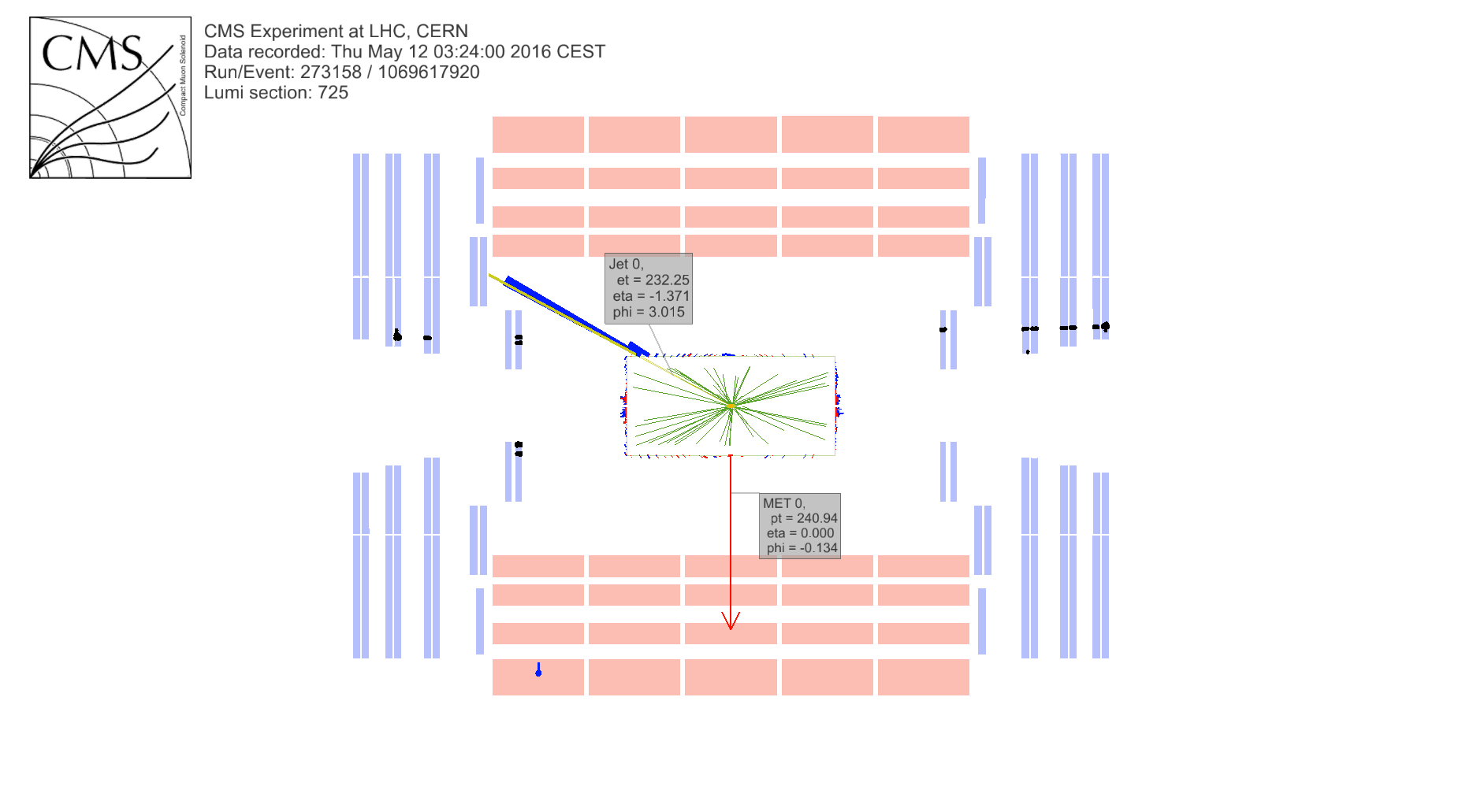
We are going to be running through parts of the open data analysis, Analysis of Higgs boson decays to two tau leptons using data and simulation of events at the CMS detector from 2012, which some of you may have done as part of the pre-exercises.

Analysis description

This analysis uses data and simulation of events at the CMS experiment from 2012 with the goal to study decays of a Higgs boson into two tau leptons in the final state of a muon lepton and a hadronically decayed tau lepton. The analysis follows loosely the setup of the official CMS analysis published in 2014.

We’ll be looking at the skimmed ROOT files, but those files can take considerable time to generate, depending on where you are and your internet connection. To save time, we’ve run Step 1 of that exercise already and generated the skimmed ROOT files. We’ve also modified some of the scripts slightly to make it easier to copy the files out of the VM/container and included some new, simpler files that allow you to inspect these ROOT files and make some first-order plots.

If you haven’t yet, you may want to check out the analysis to get a feel for the physics.

You can download the files and code by checking out the master branch of this lesson.

cd
git clone -b master git://github.com/cms-opendata-workshop/workshop-lesson-plotting-and-interpretation

This can take a few minutes as it’s about 60 MB of files.

Once it’s downloaded, you can descend into the appropriate directory. We’ll also want to make a plots directory here. The set of commands is given below.

cd workshop-lesson-plotting-and-interpretation/scripts_and_data
mkdir plots
ls -l

-rw-r--r-- 1 root root  7524470 Oct  1 05:20 DYJetsToLLSkim.root
-rw-r--r-- 1 root root   786366 Oct  1 05:20 GluGluToHToTauTauSkim.root
-rw-r--r-- 1 root root 13548245 Oct  1 05:20 Run2012B_TauPlusXSkim.root
-rw-r--r-- 1 root root 20688325 Oct  1 05:20 Run2012C_TauPlusXSkim.root
-rw-r--r-- 1 root root  4769020 Oct  1 05:20 TTbarSkim.root
-rw-r--r-- 1 root root  1156105 Oct  1 05:20 VBF_HToTauTauSkim.root
-rw-r--r-- 1 root root  3591969 Oct  1 05:20 W1JetsToLNuSkim.root
-rw-r--r-- 1 root root  5965972 Oct  1 05:20 W2JetsToLNuSkim.root
-rw-r--r-- 1 root root  3520631 Oct  1 05:20 W3JetsToLNuSkim.root
-rw-r--r-- 1 root root     3048 Oct  1 05:20 compare_two_files.py
-rw-r--r-- 1 root root     3264 Oct  1 05:20 dump_and_plot.py
-rw-r--r-- 1 root root     5864 Oct  1 05:20 histograms.py
-rw-r--r-- 1 root root     7655 Oct  1 05:20 plot.py
drwxr-xr-x 2 root root     4096 Oct  1 05:24 plots

Testing ROOT

From this directory, lets try opening one of these files, the signal Monte Carlo, GluGluToHToTauTauSkim.root.

We can do this from the ROOT C-interpreter.

root GluGluToHToTauTauSkim.root

   ------------------------------------------------------------------
  | Welcome to ROOT 6.22/02                        https://root.cern |
  | (c) 1995-2020, The ROOT Team; conception: R. Brun, F. Rademakers |
  | Built for linuxx8664gcc on Aug 18 2020, 07:08:00                 |
  | From tag , 17 August 2020                                        |
  | Try '.help', '.demo', '.license', '.credits', '.quit'/'.q'       |
   ------------------------------------------------------------------

root [0]
Attaching file GluGluToHToTauTauSkim.root as _file0...
(TFile *) 0x56356e5cf260

Testing X11 forward (for some users)

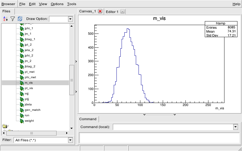
If you have been able to enable X11 forwarding, you can launch the ROOT TBrowser to inspect the ROOT file and see what is in there.

Assuming you have run the previous ROOT command and are in the CINT, you can now
root [1] TBrowser b;
And you should see the TBrowser pop up. Double-click on the GluGluToHToTauTauSkim.root and then Events and you can browse the entries and make some histograms.

Whether or not you have gotten X11 working, you can exit ROOT by typing .q.

root [2] .q

Key Points

The most straightforward way to open your skimmed files is with ROOT

There are different plotting libraries out there but you can get started pretty easily with ROOT

Make a few plots

Overview

Teaching: 10 min
Exercises: 15 min

Questions

How do I run some simple scripts?

How do I compare distributions from different files?

What am I looking at?

Objectives

Understand the basics of a simple PyROOT plotting script

Start to think about how your plots reflect the physics and the detector

What’s in these files?

Let’s use one of the provided scripts to dump the contents of the file to screen. We’ll be using a python script that calls ROOT using the PyROOT module.

cd /root/workshop-lesson-plotting-and-interpretation/scripts_and_data
python dump_and_plot.py GluGluToHToTauTauSkim.root

File**		GluGluToHToTauTauSkim.root	GluGluToHToTauTauSkim.root
 TFile*		GluGluToHToTauTauSkim.root	GluGluToHToTauTauSkim.root
  KEY: TTree	Events;1	Events
******************************************************************************
*Tree    :Events    : Events                                                 *
*Entries :     8085 : Total =         1277350 bytes  File  Size =     775872 *
*        :          : Tree compression factor =   1.63                       *
******************************************************************************
*Br    0 :njets     : njets/I                                                *
*Entries :     8085 : Total  Size=      33417 bytes  File Size  =       5961 *
*Baskets :        8 : Basket Size=      32000 bytes  Compression=   5.52     *
*............................................................................*
*Br    1 :npv       : npv/I                                                  *
*Entries :     8085 : Total  Size=      33393 bytes  File Size  =       9789 *
*Baskets :        8 : Basket Size=      32000 bytes  Compression=   3.36     *
*............................................................................*
*Br    2 :pt_1      : pt_1/F                                                 *
*Entries :     8085 : Total  Size=      33405 bytes  File Size  =      29572 *
*Baskets :        8 : Basket Size=      32000 bytes  Compression=   1.11     *
*............................................................................*
*Br    3 :eta_1     : eta_1/F                                                *
*Entries :     8085 : Total  Size=      33417 bytes  File Size  =      30766 *
*Baskets :        8 : Basket Size=      32000 bytes  Compression=   1.07     *
*............................................................................*
*Br    4 :phi_1     : phi_1/F                                                *
*Entries :     8085 : Total  Size=      33417 bytes  File Size  =      30907 *
*Baskets :        8 : Basket Size=      32000 bytes  Compression=   1.07     *
*............................................................................*
.
.
.
Br   33 :jdeta     : jdeta/F                                                *
*Entries :     8085 : Total  Size=      33417 bytes  File Size  =      13696 *
*Baskets :        8 : Basket Size=      32000 bytes  Compression=   2.40     *
*............................................................................*
*Br   34 :gen_match : gen_match/O                                            *
*Entries :     8085 : Total  Size=       9204 bytes  File Size  =        933 *
*Baskets :        8 : Basket Size=      32000 bytes  Compression=   9.33     *
*............................................................................*
*Br   35 :run       : run/I                                                  *
*Entries :     8085 : Total  Size=      33393 bytes  File Size  =       1012 *
*Baskets :        8 : Basket Size=      32000 bytes  Compression=  32.53     *
*............................................................................*
*Br   36 :weight    : weight/F                                               *
*Entries :     8085 : Total  Size=      33429 bytes  File Size  =       1071 *
*Baskets :        8 : Basket Size=      32000 bytes  Compression=  30.76     *
*............................................................................*

Wow! There’s a lot in there! We won’t go through it all now, but we know there’s information in there about some of the particles used in the analysis.

We can edit our script to loop over the individual events and make a histogram of the transverse momentum for one of the muons.

Open the dump_and_plot.py for editing using the editor of your choice. Let’s comment out the following line by placing a # in front of it.

t.Print()

Now, we’ll uncomment a big block of code that runs over the events and fills a histogram. To uncomment the code, look for three ''' that are at the beginning and end of this code block and put a # in front of them.

#'''

# Create a canvas to draw on
# canvas(name, title, x (upper corner), y (upper corner), width (pixels), height (pixels))
canvas = ROOT.TCanvas("canvas","canvas",10,10,400,400)

# Divide it into 1x1 grid
canvas.Divide(1,1)

# Create a histogram to fill for the
# TH1F(name, title, # of bins, lo edge, hi edge)
hpt_1 = ROOT.TH1F("hpt_1","Muon pT",30,0,100)

# Get the number of entries in this file
nentries = t.GetEntries()

# Loop over the entries (events/collisions)
for i in range(nentries):

    # Get each entry and fill the TTree
    t.GetEvent(i)

    # Fill the histogram with each event
    hpt_1.Fill(t.pt_1)


# Go to the first block on the canvas
canvas.cd(1)
# Draw the histogram on there
hpt_1.Draw()

# We need this line for the plot to stay active sometimes
ROOT.gPad.Update()

# Save the plot as an image. This is useful in case our
# canvas doesn't stay active
canvas.SaveAs("plots/TEST_pt_1.png")
#'''

Now we’ll run the code again. You can just repeat the same command as before, in which case it will produce a .png file that you can copy out of the environment.

Or, if you were able to get X11-forwarding working, you can run it in interactive mode, in which case a plot will pop up!

python -i dump_and_plot.py GluGluToHToTauTauSkim.root

You can exit the interactive python environment by typing

quit()

If you were not able to get X11 working, you’ll want to copy the plots subdirectory out of the environment and on to your local machine so you can inspect the figures.

If you are running Docker you can do the following on your local/host machine.

docker cp root6:/root/workshop-lesson-plotting-and-interpretation/scripts_and_data/plots .

The plots directory should now be on your local machine. In there is a file TEST_pt_1.png. It should be the same image as what popped up for some of you.

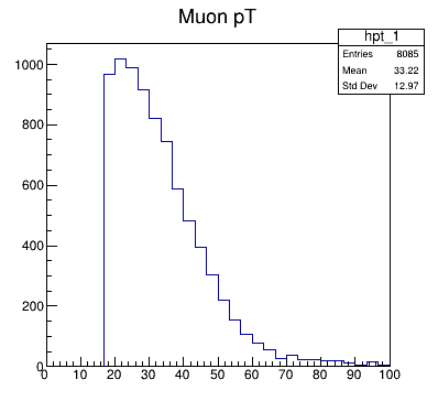
Challenge!

This is the transverse momentum for some of the muons in this analysis. Why does it have this shape? Why do you think the momentum doesn’t extend all the way down to 0?

From here on out, it will be up to you to either reference the X11-forwarded plots or go through the process of copying the plots directory on to your local machine.

More plots?

Let’s take a look at more information for these muons, specifically the transverse momentum, eta, phi, and the charge for these muons.

Let’s go back and edit the dump_and_plot.py script, and do the same commenting/uncommenting. To uncomment the code, look for three ''' that are at the beginning and end of this code block and put a # in front of them.

#'''
# Create a canvas to draw on
# canvas(name, title, x (upper corner), y (upper corner), width (pixels), height (pixels))
canvas = ROOT.TCanvas("canvas","canvas",10,10,1200,800)

# Divide it into 1x1 grid
canvas.Divide(2,2)

# Create some histograms to fill for the
# TH1F(name, title, # of bins, lo edge, hi edge)
hpt_1 = ROOT.TH1F("hpt_1","Muon pT",50,0,100)
heta_1 = ROOT.TH1F("heta_1","Muon eta",50,-3,3)
hphi_1 = ROOT.TH1F("hphi_1","Muon phi",50,-4,4)
hq_1 = ROOT.TH1F("hq_1","Muon charge",5,-2.5,2.5)

# Get the number of entries in this file
nentries = t.GetEntries()

# Loop over the entries (events/collisions)
for i in range(nentries):

    # Get each entry and fill the TTree
    t.GetEvent(i)

    # Fill the histograms as we loop over each event
    hpt_1.Fill(t.pt_1)
    heta_1.Fill(t.eta_1)
    hphi_1.Fill(t.phi_1)
    hq_1.Fill(t.q_1)

# Go to each block on the canvas and draw a histogram
canvas.cd(1)
hpt_1.Draw()

canvas.cd(2)
heta_1.Draw()

canvas.cd(3)
hphi_1.Draw()

canvas.cd(4)
hq_1.Draw()

# We need this line for the plot to stay active sometimes
ROOT.gPad.Update()

# Save the plot as an image. This is useful in case our
# canvas doesn't stay active
canvas.SaveAs("plots/TEST_muon_plots.png")

#'''

Run it on that same file.

python -i dump_and_plot.py GluGluToHToTauTauSkim.root

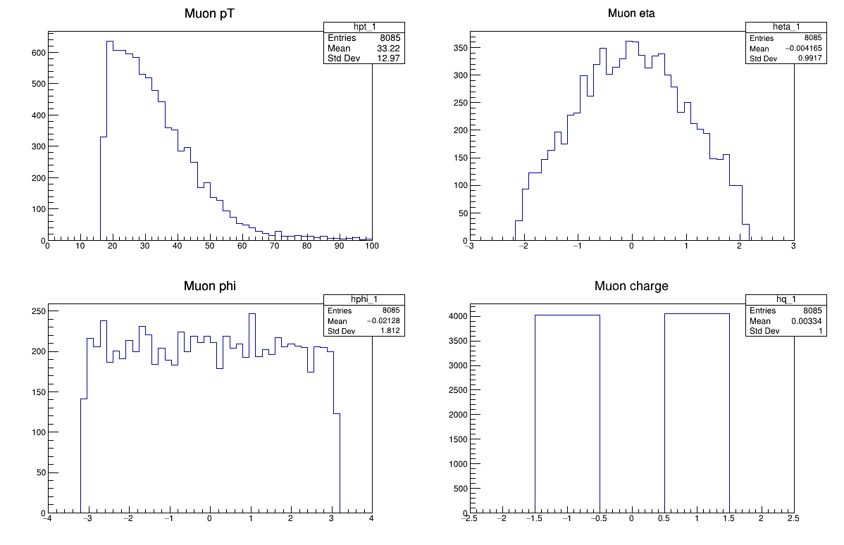
Challenge!

How about these plots? Why do they have the shapes that they do?

Hint!

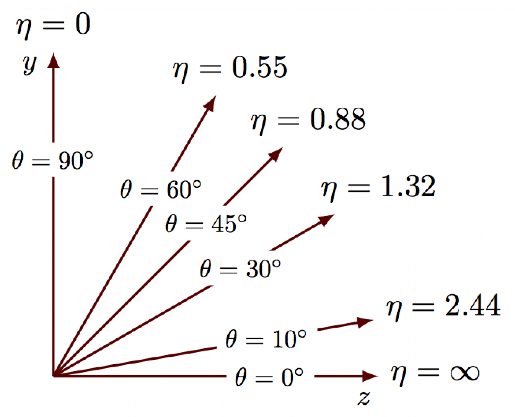
Challenge!

What about some of the other files? Do they look the same if you run on them? For example
python -i dump_and_plot.py W1JetsToLNuSkim.root

Compare some physics processes

If you ran the last challenge, you know that it would be useful to compare some of these distributions side-by-side for different physics processes.

We’ve provided a script that does this by normalizing the histograms and overlaying them. Since there are different numbers of events in each dataset, we need to normalize them for easier comparison. You won’t need to edit this script to run, but you are welcome to look at the code to get a sense of what is happening.

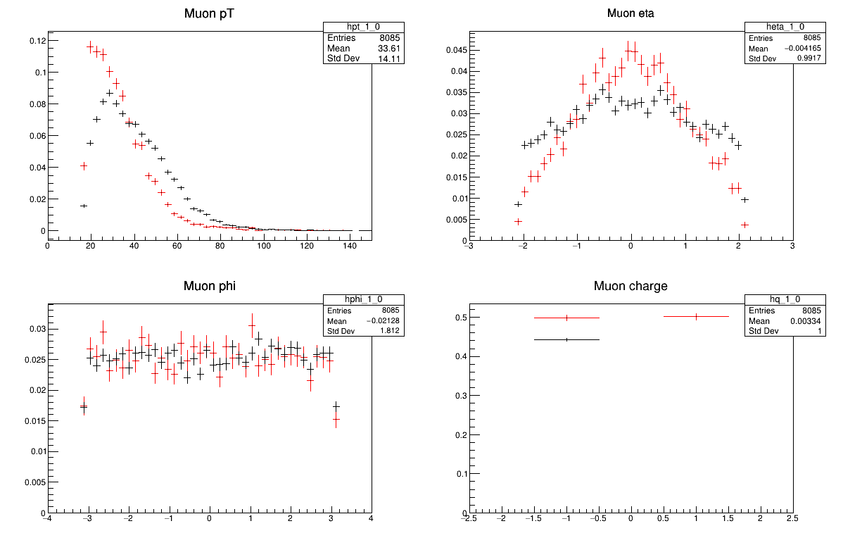
python -i compare_two_files.py GluGluToHToTauTauSkim.root W1JetsToLNuSkim.root

The red markers are the first file you pass in and the black markers are the second.

Or how about two other distributions?

python -i compare_two_files.py DYJetsToLLSkim.root TTbarSkim.root

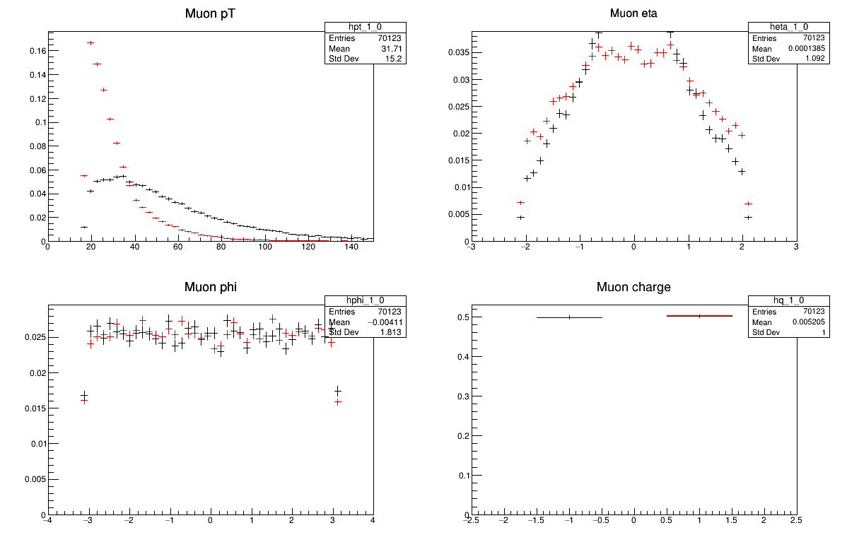
Challenge!

Why do these all look different? Is there anything you expect to be the same?

Key Points

Simple plots are often the best for first understanding of your data

Detector effects and finite acceptance will sculpt your distributions

Comparing data and Monte Carlo

Overview

Teaching: 10 min
Exercises: 10 min

Questions

How do I compare data and Monte Carlo?

What am I looking at when I do?

Objectives

Appreciate what goes into comparing data and Monte Carlo

Processing our events

In the Higgs to tau tau analysis, one runs over

Background Monte Carlo samples
The signal Monte Carlo samples
The collision data And then compares 30+ observables to see if the sum of the Monte Carlo is in agreement with the data.

In order to compare them, we need to know

What integrated luminosity does the data represent?
How many Monte Carlo events were produced?
What is the cross section for the background Monte Carlo samples?

We need those last two so we can scale the Monte Carlo to match up with the data luminosity.

That’s a lot to keep track of!

Fortunately, we’ve provided you with a script that will produce all the necessary files. In the first step, we run over all our datasets and produce ROOT files that contain the histograms of our 30+ observables, weighted appropriately.

We can run this as follows.

cd /root/workshop-lesson-plotting-and-interpretation/scripts_and_data
python histograms.py 

.
.
<warnings we can ignore> 
.
.
>> Process skimmed sample GluGluToHToTauTau for process ggH
Cut-flow report (signal region):
Muon transverse mass cut for W+jets suppression: pass=5591       all=8085       -- eff=69.15 % cumulative eff=69.15 %
Require isolated muon for signal region: pass=4990       all=5591       -- eff=89.25 % cumulative eff=61.72 %
Require opposited charge for signal region: pass=4913       all=4990       -- eff=98.46 % cumulative eff=60.77 %
Cut-flow report (control region):
Muon transverse mass cut for W+jets suppression: pass=5591       all=8085       -- eff=69.15 % cumulative eff=69.15 %
Require isolated muon for signal region: pass=4990       all=5591       -- eff=89.25 % cumulative eff=61.72 %
Control region for QCD estimation: pass=77         all=4990       -- eff=1.54 % cumulative eff=0.95 %
>>> Process skimmed sample VBF_HToTauTau for process qqH
Cut-flow report (signal region):
Muon transverse mass cut for W+jets suppression: pass=7129       all=10492      -- eff=67.95 % cumulative eff=67.95 %
Require isolated muon for signal region: pass=6562       all=7129       -- eff=92.05 % cumulative eff=62.54 %
Require opposited charge for signal region: pass=6420       all=6562       -- eff=97.84 % cumulative eff=61.19 %
Cut-flow report (control region):
Muon transverse mass cut for W+jets suppression: pass=7129       all=10492      -- eff=67.95 % cumulative eff=67.95 %
Require isolated muon for signal region: pass=6562       all=7129       -- eff=92.05 % cumulative eff=62.54 %
Control region for QCD estimation: pass=142        all=6562       -- eff=2.16 % cumulative eff=1.35 %
.
.
.
>>> Process skimmed sample Run2012B_TauPlusX for process dataRunB
Cut-flow report (signal region):
Muon transverse mass cut for W+jets suppression: pass=64837      all=136060     -- eff=47.65 % cumulative eff=47.65 %
Require isolated muon for signal region: pass=37378      all=64837      -- eff=57.65 % cumulative eff=27.47 %
Require opposited charge for signal region: pass=28309      all=37378      -- eff=75.74 % cumulative eff=20.81 %
Cut-flow report (control region):
Muon transverse mass cut for W+jets suppression: pass=64837      all=136060     -- eff=47.65 % cumulative eff=47.65 %
Require isolated muon for signal region: pass=37378      all=64837      -- eff=57.65 % cumulative eff=27.47 %
Control region for QCD estimation: pass=9069       all=37378      -- eff=24.26 % cumulative eff=6.67 %
>>> Process skimmed sample Run2012C_TauPlusX for process dataRunC
Cut-flow report (signal region):
Muon transverse mass cut for W+jets suppression: pass=99497      all=210462     -- eff=47.28 % cumulative eff=47.28 %
Require isolated muon for signal region: pass=60162      all=99497      -- eff=60.47 % cumulative eff=28.59 %
Require opposited charge for signal region: pass=45644      all=60162      -- eff=75.87 % cumulative eff=21.69 %
Cut-flow report (control region):
Muon transverse mass cut for W+jets suppression: pass=99497      all=210462     -- eff=47.28 % cumulative eff=47.28 %
Require isolated muon for signal region: pass=60162      all=99497      -- eff=60.47 % cumulative eff=28.59 %
Control region for QCD estimation: pass=14518      all=60162      -- eff=24.13 % cumulative eff=6.90 %

This produces a file histograms.root that has all these histograms in it. We can examine this with ROOT, even without X11 forwarding.

root histograms.root

Once we’re in the ROOT CINT, we can do the following to see all the histograms in there!

_file0->ls()

TFile**		histograms.root
 TFile*		histograms.root
  KEY: TH1D	ggH_pt_1;1	pt_1
  KEY: TH1D	ggH_pt_2;1	pt_2
  KEY: TH1D	ggH_eta_1;1	eta_1
  KEY: TH1D	ggH_eta_2;1	eta_2
  KEY: TH1D	ggH_phi_1;1	phi_1
  KEY: TH1D	ggH_phi_2;1	phi_2
  KEY: TH1D	ggH_iso_1;1	iso_1
  KEY: TH1D	ggH_iso_2;1	iso_2
  KEY: TH1D	ggH_q_1;1	q_1
  KEY: TH1D	ggH_q_2;1	q_2
  KEY: TH1D	ggH_pt_met;1	pt_met
  KEY: TH1D	ggH_phi_met;1	phi_met
.
.
.
 KEY: TH1D	qqH_phi_met_cr;1	phi_met
  KEY: TH1D	qqH_m_1_cr;1	m_1
  KEY: TH1D	qqH_m_2_cr;1	m_2
  KEY: TH1D	qqH_mt_1_cr;1	mt_1
  KEY: TH1D	qqH_mt_2_cr;1	mt_2
  KEY: TH1D	qqH_dm_2_cr;1	dm_2
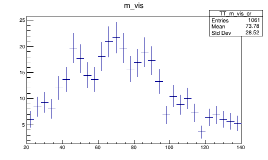
  KEY: TH1D	qqH_m_vis_cr;1	m_vis
  KEY: TH1D	qqH_pt_vis_cr;1	pt_vis
  KEY: TH1D	qqH_jpt_1_cr;1	jpt_1
  KEY: TH1D	qqH_jpt_2_cr;1	jpt_2
  KEY: TH1D	qqH_jeta_1_cr;1	jeta_1
  KEY: TH1D	qqH_jeta_2_cr;1	jeta_2
  KEY: TH1D	qqH_jphi_1_cr;1	jphi_1
  KEY: TH1D	qqH_jphi_2_cr;1	jphi_2
  KEY: TH1D	qqH_jm_1_cr;1	jm_1
  KEY: TH1D	qqH_jm_2_cr;1	jm_2
  KEY: TH1D	qqH_jbtag_1_cr;1	jbtag_1
  KEY: TH1D	qqH_jbtag_2_cr;1	jbtag_2
  KEY: TH1D	qqH_npv_cr;1	npv
  KEY: TH1D	qqH_njets_cr;1	njets
  KEY: TH1D	qqH_mjj_cr;1	mjj
  KEY: TH1D	qqH_ptjj_cr;1	ptjj
  KEY: TH1D	qqH_jdeta_cr;1	jdeta

We can look at one of these histograms, but on it’s own it’s not that interesting.

Compare Monte Carlo and data

Now we want to compare Monte Carlo and data but we need to label everything correctly and keep track of things carefully and that’s really hard! Fortunately, we’ve provided you with a script. Just like the previous command, the expected input filename is hardcoded.

python plot.py

Info in <TCanvas::Print>: pdf file plots/pt_1.pdf has been created
Info in <TCanvas::Print>: png file plots/pt_1.png has been created
Info in <TCanvas::Print>: pdf file plots/pt_2.pdf has been created
Info in <TCanvas::Print>: png file plots/pt_2.png has been created
Info in <TCanvas::Print>: pdf file plots/eta_1.pdf has been created
Info in <TCanvas::Print>: png file plots/eta_1.png has been created
Info in <TCanvas::Print>: pdf file plots/eta_2.pdf has been created
Info in <TCanvas::Print>: png file plots/eta_2.png has been created
Info in <TCanvas::Print>: pdf file plots/phi_1.pdf has been created
Info in <TCanvas::Print>: png file plots/phi_1.png has been created
Info in <TCanvas::Print>: pdf file plots/phi_2.pdf has been created
Info in <TCanvas::Print>: png file plots/phi_2.png has been created
Info in <TCanvas::Print>: pdf file plots/pt_met.pdf has been created
Info in <TCanvas::Print>: png file plots/pt_met.png has been created
Info in <TCanvas::Print>: pdf file plots/phi_met.pdf has been created
Info in <TCanvas::Print>: png file plots/phi_met.png has been created
.
.
.
Info in <TCanvas::Print>: png file plots/jphi_2.png has been created
Info in <TCanvas::Print>: pdf file plots/jm_1.pdf has been created
Info in <TCanvas::Print>: png file plots/jm_1.png has been created
Info in <TCanvas::Print>: pdf file plots/jm_2.pdf has been created
Info in <TCanvas::Print>: png file plots/jm_2.png has been created
Info in <TCanvas::Print>: pdf file plots/jbtag_1.pdf has been created
Info in <TCanvas::Print>: png file plots/jbtag_1.png has been created
Info in <TCanvas::Print>: pdf file plots/jbtag_2.pdf has been created
Info in <TCanvas::Print>: png file plots/jbtag_2.png has been created
Info in <TCanvas::Print>: pdf file plots/npv.pdf has been created
Info in <TCanvas::Print>: png file plots/npv.png has been created
Info in <TCanvas::Print>: pdf file plots/njets.pdf has been created
Info in <TCanvas::Print>: png file plots/njets.png has been created

Now we can take a look and see how good the comparison is!

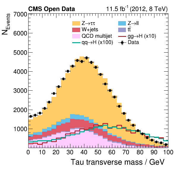
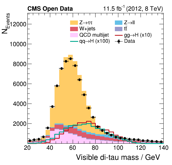
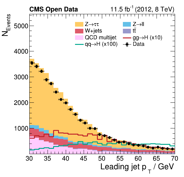
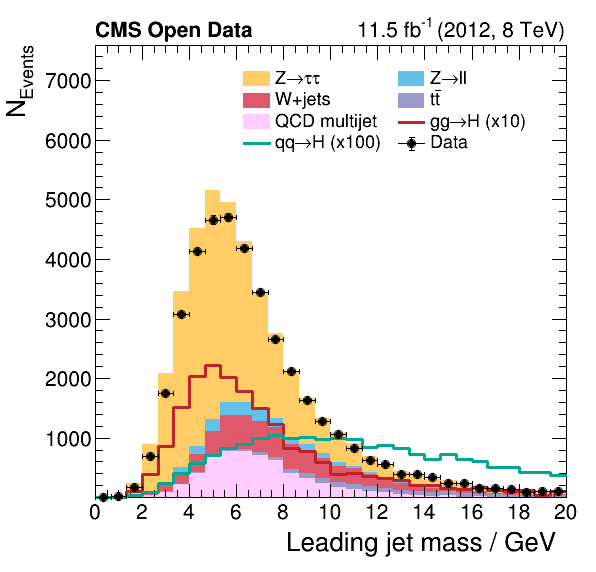
Pretty good agreement! However, for a full analysis, there’s more to be done. From the open data portal record…

More to do!

For completeness, the following points describe the missing steps to extract from the data a meaningful statistical result. Please note that these steps typically take most of the time of a physics analysis and are not included in this example.

The simulation has to be improved with corrections to reflect the data precisely. For example, a typical correction is the calibration of the energy measurement of tau leptons or jets. Each correction comes with a systematic uncertainty, which has to be included in the measurement.

As the final step, a measurement is performed with a fit of a statistical model to the data. This model incorporates the expectation from a physics model, for example the Standard Model, and all statistical and systematic uncertainties. Typical systematic uncertainties are the uncertainties of the amount of expected background events or the theory of the physics model.

But that’s for another time!

Key Points

When comparing data and Monte Carlo, there’s a lot to keep track of

Eventually, one would want to perform a fit, but that would be for another lesson

Plotting and interpretation

Introduction

Overview

Setting up a ROOT environment

Workflow for this lesson

Docker-specific commands for X11 forwarding and other miscellany

VM-specific commands go here

Download the files and code we’ll use

Analysis description

Testing ROOT

Testing X11 forward (for some users)

Key Points

Make a few plots

Overview

What’s in these files?

Challenge!

More plots?

Challenge!

Hint!

Challenge!

Compare some physics processes

Challenge!

Key Points

Comparing data and Monte Carlo

Overview

Processing our events

Compare Monte Carlo and data

More to do!

Key Points