CMS Physics Objects

Overview

Teaching: 10 min
Exercises: min

Questions

What are the main CMS Physics Objects and how do I access them?

Objectives

Identify CMS physics objects

Identify object code collections in AOD files

Access an object code collection

CMS uses the phrase “physics objects” to speak broadly about particles that can be identified via signals from the CMS detector. A physics object typically began as a single particle, but may have showered into many particles as it traversed the detector. The principle physics objects are:

muons
electrons
taus
photons
jets
missing transverse momentum

Viewing modules in a data file

CMS AOD files store all physics objects of the same type in “modules”. These modules are data structures that act as containers for multiple instances of the same C++ class. The edmDumpEventContent command show below lists all the modules in a file. As an example, the “muons” module in AOD contains many reco::Muon objects (one per muon in the event).

$ edmDumpEventContent root://eospublic.cern.ch//eos/opendata/cms/MonteCarlo2012/Summer12_DR53X/TTbar_8TeV-Madspin_aMCatNLO-herwig/AODSIM/PU_S10_START53_V19-v2/00000/000A9D3F-CE4C-E311-84F8-001E673969D2.root

Type                                  Module                      Label             Process
----------------------------------------------------------------------------------------------
...
vector<reco::Muon>                    "muons"                     ""                "RECO"
vector<reco::Muon>                    "muonsFromCosmics"          ""                "RECO"
vector<reco::Muon>                    "muonsFromCosmics1Leg"      ""                "RECO"
...
vector<reco::Track>                   "cosmicMuons"               ""                "RECO"
vector<reco::Track>                   "cosmicMuons1Leg"           ""                "RECO"
vector<reco::Track>                   "globalCosmicMuons"         ""                "RECO"
vector<reco::Track>                   "globalCosmicMuons1Leg"     ""                "RECO"
vector<reco::Track>                   "globalMuons"               ""                "RECO"
vector<reco::Track>                   "refittedStandAloneMuons"   ""                "RECO"
vector<reco::Track>                   "standAloneMuons"           ""                "RECO"
vector<reco::Track>                   "refittedStandAloneMuons"   "UpdatedAtVtx"    "RECO"
vector<reco::Track>                   "standAloneMuons"           "UpdatedAtVtx"    "RECO"
vector<reco::Track>                   "tevMuons"                  "default"         "RECO"
vector<reco::Track>                   "tevMuons"                  "dyt"             "RECO"
vector<reco::Track>                   "tevMuons"                  "firstHit"        "RECO"
vector<reco::Track>                   "tevMuons"                  "picky"           "RECO"

Note that this file also contains many other muon-related modules: two modules of reco::Muon muons from cosmic-ray events, and many modules of reco::Track objects that give lower-level tracking information for muons. As you can see, the AOD file contains MANY modules, and not all of them are related directly to physics objects. Other important modules might include:

Tracks and vertices
Calorimeter clusters and other detector information
Particle Flow candidates
Triggers
Pileup (info about multiple collisions from the same pp crossing)
Generator-level information (in simulation)

Opening a module

Setup

The AOD2NanoAODOutreachTool repository is the example we will use for accessing information from AOD files. If you have not already done so, please check out the “dummyworkshop” branch of this repository:
$ cd ~/CMSSW_5_3_32/src/
$ cmsenv
$ mkdir workspace
$ cd workspace
$ git clone -b dummyworkshop git://github.com/jmhogan/AOD2NanoAODOutreachTool.git 
$ cd AOD2NanoAODOutreachTool
$ scram b
$ vi src/AOD2NanoAOD.cc #(or your favorite text editor)

In the source code for this tool, the definitions of the muon classes are included:

#include "DataFormats/MuonReco/interface/Muon.h"
#include "DataFormats/MuonReco/interface/MuonFwd.h"
#include "DataFormats/MuonReco/interface/MuonSelectors.h"

You learned about the EDAnalyzer class in the pre-exercises. The AOD2NanoAOD tool is an EDAnalyzer. The “analyze” function of an EDAnalyzer is performed once per event. Muons can be accessed like this:

void AOD2NanoAOD::analyze(const edm::Event &iEvent,
                          const edm::EventSetup &iSetup) {

  using namespace edm;
  using namespace reco;
  using namespace std;

  Handle<MuonCollection> muons;
  iEvent.getByLabel(InputTag("muons"), muons);

The result is an called “muons” which is a collection of all the muon objects. In the next episode we’ll look at the member functions for muons. Collection classes are generally constructed as std::vectors. We can quickly access the number of muons per event and create a loop to access individual muons:

int nMuons = muons->size();
for (auto it = muons->begin(); it != muons->end(); it++) {
    if (it->pt() > mu_min_pt) {
        // do things here, next episode!
    }
}

Key Points

CMS physics objects include: muons, electrons, taus, photons, and jets.

Missing transverse momentum is derived from physics objects (negative vector sum).

Objects are stored in separate collections in the AOD files

Objects can be accessed one-by-one via a for loop

Accessing common quantities

Overview

Teaching: 15 min
Exercises: 30 min

Questions

How can I store basic information about a given object, like 4-vectors?

Objectives

Learn member functions for standard momentum-energy vectors

Learn member functions for common track-based quantities

Learn how to connect a physics object with a generator-level particle

Practice accessing and saving these quantities

Many of the most important kinematic quantities defining a physics object are accessed in a common way across all the objects. All objects have associated energy-momentum vectors, typically constructed using transverse momentum, pseudorapdity, azimuthal angle, and mass or energy.

4-vector access functions

In AOD2NanoAOD/src/AOD2NanoAOD.cc the muon four-vector elements are accessed as shown below. The values for each muon are stored into an array, which will become a branch in a ROOT TTree.

for (auto it = muons->begin(); it != muons->end(); it++) {
  value_mu_pt[value_mu_n] = it->pt();
  value_mu_eta[value_mu_n] = it->eta();
  value_mu_phi[value_mu_n] = it->phi();
  value_mu_mass[value_mu_n] = it->mass();
}

Challenge: electron 4-vector

You set up the workshop’s version of the AOD2NanoAOD tool in the previous episode. Now edit src/AOD2NanoAOD.cc to access and store the electron’s four-vector elements, folling the examples set for muons. Note: You’ll also need to create the arrays and TTree branches!
Solution:

There are 3 elements to add: declarations, branches, and accessing values. Declare the variables near the top of the file with other similar statements:
float value_el_pt[max_el];
float value_el_eta[max_el];
float value_el_phi[max_el];
float value_el_mass[max_el];
Add branches to the tree after declaring the variables. The first argument is the branch name, the second argument is the variable to be stored in this branch, and the third argument gives the branch’s structure as an array of floats (/f) with size [nElectron].
tree->Branch("electron_pt", value_el_pt, "electron_pt[nElectron]/f");
tree->Branch("electron_eta", value_el_eta, "electron_eta[nElectron]/f");
tree->Branch("electron_phi", value_el_phi, "electron_phi[nElectron]/f");
tree->Branch("electron_mass", value_el_mass, "electron_mass[nElectron]/f");
Finally, in the loop over the electron collection, access the elements of the four-vector:
value_el_pt[value_el_n] = it->pt();
value_el_eta[value_el_n] = it->eta();
value_el_phi[value_el_n] = it->phi();
value_el_mass[value_el_n] = it->mass();

Track access functions

Many objects are also connected to tracks from the CMS tracking detectors. Information from tracks provides other kinematic quantities that are common to multiple types of objects.

From a muon object, we can access the electric charge and the associated track:

value_mu_charge[value_mu_n] = it->charge();
auto trk = it->globalTrack(); // muon track

Often, the most pertinent information about an object (such as a muon) to access from its associated track is its impact parameter with respect to the primary interaction vertex. Since muons can also be tracked through the muon detectors, we first check if the track is well-defined, and then access impact parameters in the xy-plane (dxy or d0) and along the beam axis (dz), as well as their respective uncertainties.

if (trk.isNonnull()) {
   value_mu_dxy[value_mu_n] = trk->dxy(pv);
   value_mu_dz[value_mu_n] = trk->dz(pv);
   value_mu_dxyErr[value_mu_n] = trk->d0Error();
   value_mu_dzErr[value_mu_n] = trk->dzError();
}

Challenge: electron track properties

Access and store the electron’s charge and track impact parameter values, following the examples set for muons. Electron tracks are found using the Gaussian-sum filter method, which influences the member function name to access the track:
auto trk = it->gsfTrack(); // electron track
Solution:

Again, add information in three places: Declarations:
int value_el_charge[max_el];
float value_el_dxy[max_el];
float value_el_dxyErr[max_el];
float value_el_dz[max_el];
float value_el_dzErr[max_el];
Branches:
tree->Branch("Electron_charge", value_el_charge, "Electron_charge[nElectron]/I");
tree->Branch("Electron_dxy", value_el_dxy, "Electron_dxy[nElectron]/F");
tree->Branch("Electron_dxyErr", value_el_dxyErr, "Electron_dxyErr[nElectron]/F");
tree->Branch("Electron_dz", value_el_dz, "Electron_dz[nElectron]/F");
tree->Branch("Electron_dzErr", value_el_dzErr, "Electron_dzErr[nElectron]/F");
And access values in the electron loop. The format is identical to the muon loop!
value_el_charge[value_el_n] = it->charge();

auto trk = it->gsfTrack();
value_el_dxy[value_el_n] = trk->dxy(pv);
value_el_dz[value_el_n] = trk->dz(pv);
value_el_dxyErr[value_el_n] = trk->d0Error();
value_el_dzErr[value_el_n] = trk->dzError();

Matching to generated particles

Simulated files also contain information about the generator-level particles that were propagated into the showering and detector simulations. Physics objects can be matched to these generated particles spatially.

The AOD2NanoAOD tool sets up several utility functions for matching: findBestMatch, findBestVisibleMatch, and subtractInvisible. The findBestMatch function takes generated particles (with an automated type T) and the 4-vector of a physics object. It uses angular separation to find the closest generated particle to the reconstructed particle:

template <typename T>
int findBestMatch(T& gens, reco::Candidate::LorentzVector& p4) {

  # initial definition of "closest" is really bad
  float minDeltaR = 999.0;
  int idx = -1;

  # loop over the generated particles
  for (auto g = gens.begin(); g != gens.end(); g++) {
    const auto tmp = deltaR(g->p4(), p4);

    # if it's closer, overwrite the definition of "closest"
    if (tmp < minDeltaR) {
      minDeltaR = tmp;
      idx = g - gens.begin();
    }
  }
  return idx; # return the index of the match
}

The other utility functions are similar, but correct for generated particles that decay to neutrinos, which would affect the “visible” 4-vector.

In the AOD2NanoAOD tool, muons are matched only to “interesting” generated particles, which are all the leptons and photons (PDG ID 11, 13, 15, 22). Their generator status must be 1, indicating a final-state particle after any radiation chain.

if (!isData){
   value_gen_n = 0;
   
   for (auto p = selectedMuons.begin(); p != selectedMuons.end(); p++) {

      // get the muon's 4-vector
      auto p4 = p->p4();

      // perform the matching with a utility function
      auto idx = findBestVisibleMatch(interestingGenParticles, p4);

      // if a match was found, save the generated particle's information
      if (idx != -1) {
      	 auto g = interestingGenParticles.begin() + idx;

	 // another example of common 4-vector access functions!
         value_gen_pt[value_gen_n] = g->pt();
         value_gen_eta[value_gen_n] = g->eta();
         value_gen_phi[value_gen_n] = g->phi();
         value_gen_mass[value_gen_n] = g->mass();

	 // gen particles also have ID and status from the generator
         value_gen_pdgid[value_gen_n] = g->pdgId();
         value_gen_status[value_gen_n] = g->status();

	 // save the index of the matched gen particle
         value_mu_genpartidx[p - selectedMuons.begin()] = value_gen_n;
         value_gen_n++;
      }
   }
}

Challenge: electron matching

Match selected electrons to the interesting generated particles. Compile your code and run over the simulation test file. Using the ROOT TBrowser, look at some histograms of the branches you’ve added to the tree throughout this episode.
$ scram b
$ cmsRun configs/simulation_cfg.py
$ root -l output.root
[1] TBrowser b
Solution:

The structure for this matching exercise is identical to the muon matching segment. Loop over selected electrons, use the findBestVisibleMatch function to match it to an “interesting” particle and then to a jet.
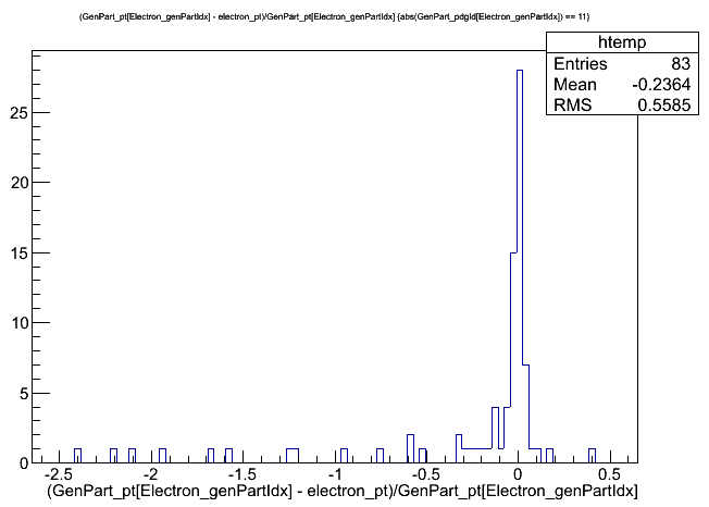
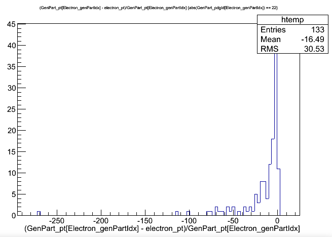
// Match electrons with gen particles and jets
for (auto p = selectedElectrons.begin(); p != selectedElectrons.end(); p++) {
 // Gen particle matching
 auto p4 = p->p4();
 auto idx = findBestVisibleMatch(interestingGenParticles, p4);
 if (idx != -1) {
   auto g = interestingGenParticles.begin() + idx;
   value_gen_pt[value_gen_n] = g->pt();
   value_gen_eta[value_gen_n] = g->eta();
   value_gen_phi[value_gen_n] = g->phi();
   value_gen_mass[value_gen_n] = g->mass();
   value_gen_pdgid[value_gen_n] = g->pdgId();
   value_gen_status[value_gen_n] = g->status();
   value_el_genpartidx[p - selectedElectrons.begin()] = value_gen_n;
   value_gen_n++;
 }

 // Jet matching
 value_el_jetidx[p - selectedElectrons.begin()] = findBestMatch(selectedJets, p4);
}
As an example of using these new branches, we can plot the electrons’ pT resolution and compare cases where the electrons were matched to a generated electron, vs where they were matched to a photon. Unsurprisingly, the resolution is much smaller for properly gen-matched electrons!
$ root -l output.root
[1] _file0->cd("aod2nanoaod")
[2] Events->Draw("(GenPart_pt[Electron_genPartIdx] - electron_pt)/GenPart_pt[Electron_genPartIdx]","abs(GenPart_pdgId[Electron_genPartIdx]) == 11");
[3] Events->Draw("(GenPart_pt[Electron_genPartIdx] - electron_pt)/GenPart_pt[Electron_genPartIdx]","abs(GenPart_pdgId[Electron_genPartIdx]) == 22");

Key Points

Physics objects in CMS inherit common member functions for the 4-vector quantities of transverse momentum, polar/azimuthal angles, and mass/energy.

Objects are matched to generator-level particles based on spatial relationships.

Other quantities such as impact parameters and charge have common member functions.

Accessing CMS-specific object information

Overview

Teaching: 15 min
Exercises: 30 min

Questions

Where can I find CMS-specific information about a given object, like identification criteria?

Objectives

Bookmark informational web pages for different objects

Learn member functions for identification and isolation of objects

Learn member functions for detector-related quantities

Practice accessing and saving these quantities

When is a muon not a muon? How do we guarantee that signals from the muon detector correspond to a “real” muon? How do we distinguish between muons produced directly from decays of more massive particles (ex: $H \rightarrow 4\mu$) from muons produced in semi-leptonic decays of heavy quarks?

The most signicant difference between a list of certain particles from a Monte Carlo generator and a list of the corresponding physics objects from CMS is likely the inherent uncertainty in the reconstruction. Selection of “a muon” or “an electron” for analysis requires algorithms designed to separate “real” objects from “fakes”. These are called identification algorithms.

Other algorithms are designed to measure the amount of energy deposited near the object, to determine if it was likely produced near the primary interaction (typically little nearby energy), or from the decay of a longer-lived particle (typically a lot of nearby energy). These are called isolation algorithms. Many types of isolation algorithms exist to deal with unique physics cases!

Both types of algorithms function using working points that are described on a spectrum from “loose” to “tight”. Working points that are “looser” tend to have a high efficiency for accepting real objects, but perhaps a poor rejection rate for “fake” objects. Working points that are “tighter” tend to have lower efficiencies for accepting real objects, but much better rejection rates for “fake” objects. The choice of working point is highly analysis dependent! Some analyses value efficiency over background rejection, and some analyses are the opposite.

The “standard” identification and isolation algorithm results can be accessed from the physics object classes. CMS maintains reference pages that document the various options:

General: CMS Physics Objects 2011
Muons: SWGuide Muon ID
Electrons: EGamma Public Data
Photons: EGamma Public Data, Summary document (see Table 1 for photon ID)
Tau leptons: Legacy Tau ID Run 1, Nutshell Recipe

Muons

The CMS Muon object group has created member functions for the identification algorithms that simply storing pass/fail decisions about the quality of each muon. As shown below, the algorithm depends on which vertex is being considered as the primary interaction vertex!

Hard processes produce large angles between the final state partons. The final object of interest will be separated from the other objects in the event or be “isolated”. For instance, an isolated muon might be produced in the decay of a W boson. In contrast, a non-isolated muon can come from a weak decay inside a jet.

Muon isolation is calculated from a combination of factors: energy from charged hadrons, energy from neutral hadrons, and energy from photons, all in a cone of radius $\Delta R < 0.3$ or 0.4 around the muon. Many algorithms also feature a “correction factor” that subtracts average energy expected from pileup contributions to this cone. Decisions are made by comparing this energy sum to the transverse momentum of the muon.

for (auto it = muons->begin(); it != muons->end(); it++) {

    // If this muon has isolation quantities...
    if (it->isPFMuon() && it->isPFIsolationValid()) {

       // get the isolation info in a certain cone size:
       auto iso04 = it->pfIsolationR04();

       // and calculate the energy relative to the muon's transverse momentum
       value_mu_pfreliso04all[value_mu_n] = (iso04.sumChargedHadronPt + iso04.sumNeutralHadronEt + iso04.sumPhotonEt)/it->pt();
    }

    // Store the pass/fail decisions about Tight ID
    value_mu_tightid[value_mu_n] = muon::isTightMuon(*it, *vertices->begin());
}

Challenge: alternate IDs and isolations

Using the documentation on the TWiki page, adjust the 0.4-cone muon isolation calculation to apply the “DeltaBeta” pileup correction. Also add the pass/fail information about the Loose and Soft identification working points.
Solution:

The DeltaBeta correction for pileup involves subtracting off half of the pileup contribution that can be accessed from the “iso04” object already being used:
value_mu_pfreliso04all[value_mu_n] =
   (iso04.sumChargedHadronPt + max(0.,iso04.sumNeutralHadronEt + iso04.sumPhotonEt- 0.5*iso04.sumPUPt))/it->pt();
To add new ID variables we follow the same sequence as other challenges: declaration, branch, access. You might add these beneath the existing “Tight” ID in all three places:
bool value_mu_tightid[max_mu];
bool value_mu_softid[max_mu];
bool value_mu_looseid[max_mu];
tree->Branch("Muon_tightId", value_mu_tightid, "Muon_tightId[nMuon]/O");
tree->Branch("Muon_softId", value_mu_softid, "Muon_softId[nMuon]/O");
tree->Branch("Muon_looseId", value_mu_looseid, "Muon_looseId[nMuon]/O");
value_mu_tightid[value_mu_n] = muon::isTightMuon(*it, *vertices->begin());
value_mu_softid[value_mu_n] = muon::isSoftMuon(*it, *vertices->begin());
value_mu_looseid[value_mu_n] = muon::isLooseMuon(*it);

Tau leptons

The CMS Tau object group relies almost entirely on pre-computed algorithms to determine the quality of the tau reconstruction and the decay type. Since this object is not stable and has several decay modes, different combinations of identification and isolation algorithms are used across different analyses. The TWiki page provides a large table of available algorithms.

In contrast to the muon object, tau algorithm results are typically saved in the AOD files as their own PFTauDisciminator collections, rather than as part of the tau object class.

// Get the tau collection
Handle<PFTauCollection> taus;
iEvent.getByLabel(InputTag("hpsPFTauProducer"), taus);

// Get various tau discriminator collections
Handle<PFTauDiscriminator> tausLooseIso, tausVLooseIso, tausMediumIso, tausTightIso,
                           tausDecayMode, tausRawIso;

iEvent.getByLabel(InputTag("hpsPFTauDiscriminationByDecayModeFinding"),tausDecayMode);
iEvent.getByLabel(InputTag("hpsPFTauDiscriminationByRawCombinedIsolationDBSumPtCorr"),tausRawIso);
iEvent.getByLabel(InputTag("hpsPFTauDiscriminationByVLooseCombinedIsolationDBSumPtCorr"),tausVLooseIso);
//...etc...

The tau discriminator collections act as pairs, containing the index of the tau and the value of the discriminant for that tau. Note that the arrays are filled by calls to the individual discriminant objects, but referencing the vector index of the tau in the main tau collection.

for (auto it = taus->begin(); it != taus->end(); it++) {

    // store the tau decay mode
    value_tau_decaymode[value_tau_n] = it->decayMode();

    // Discriminators
    const auto idx = it - taus->begin();
    value_tau_iddecaymode[value_tau_n] = tausDecayMode->operator[](idx).second;
    value_tau_idisoraw[value_tau_n] = tausRawIso->operator[](idx).second;
    value_tau_idisovloose[value_tau_n] = tausVLooseIso->operator[](idx).second;
    // ...etc...
}

Challenge: alternate tau IDs

Many other tau discriminants exist. Based on information from the TWiki, save the values for some discriminants that are based on rejecting electrons or muons.

Solution:

The TWiki describes Loose/Medium/Tight ID levels for an “AntiElectron” algorithm and an “AntiMuon” algorithm. They can be accessed like the other tau IDs, but you might need to refer to the output of edmDumpEventContent to find the exact form of the InputTag name.

Add declarations:

bool value_tau_idantieleloose[max_tau];
bool value_tau_idantielemedium[max_tau];
bool value_tau_idantieletight[max_tau];
bool value_tau_idantimuloose[max_tau];
bool value_tau_idantimumedium[max_tau];
bool value_tau_idantimutight[max_tau];

Add branches:

tree->Branch("Tau_idAntiEleLoose", value_tau_idantieleloose, "Tau_idAntiEleLoose[nTau]/O");
tree->Branch("Tau_idAntiEleMedium", value_tau_idantielemedium, "Tau_idAntiEleMedium[nTau]/O");
tree->Branch("Tau_idAntiEleTight", value_tau_idantieletight, "Tau_idAntiEleTight[nTau]/O");
tree->Branch("Tau_idAntiMuLoose", value_tau_idantimuloose, "Tau_idAntiMuLoose[nTau]/O");
tree->Branch("Tau_idAntiMuMedium", value_tau_idantimumedium, "Tau_idAntiMuMedium[nTau]/O");
tree->Branch("Tau_idAntiMuTight", value_tau_idantimutight, "Tau_idAntiMuTight[nTau]/O");

Create handles and get the information from the input file:

Handle<PFTauCollection> taus;
iEvent.getByLabel(InputTag("hpsPFTauProducer"), taus);

Handle<PFTauDiscriminator> tausLooseIso, tausVLooseIso, tausMediumIso, tausTightIso,
                          tausDecayMode, tausLooseEleRej, tausMediumEleRej,
                          tausTightEleRej, tausLooseMuonRej, tausMediumMuonRej,
                          tausTightMuonRej, tausRawIso;

// new things only
iEvent.getByLabel(InputTag("hpsPFTauDiscriminationByLooseElectronRejection"),
       tausLooseEleRej);
iEvent.getByLabel(InputTag("hpsPFTauDiscriminationByMediumElectronRejection"),
       tausMediumEleRej);
iEvent.getByLabel(InputTag("hpsPFTauDiscriminationByTightElectronRejection"),
       tausTightEleRej);

iEvent.getByLabel(InputTag("hpsPFTauDiscriminationByLooseMuonRejection"),
       tausLooseMuonRej);
iEvent.getByLabel(InputTag("hpsPFTauDiscriminationByMediumMuonRejection"),
       tausMediumMuonRej);
iEvent.getByLabel(InputTag("hpsPFTauDiscriminationByTightMuonRejection"),
       tausTightMuonRej);

And finally, access the discriminator from the second element of the pair:

value_tau_idantieleloose[value_tau_n] = tausLooseEleRej->operator[](idx).second;
value_tau_idantielemedium[value_tau_n] = tausMediumEleRej->operator[](idx).second;
value_tau_idantieletight[value_tau_n] = tausTightEleRej->operator[](idx).second;
value_tau_idantimuloose[value_tau_n] = tausLooseMuonRej->operator[](idx).second;
value_tau_idantimumedium[value_tau_n] = tausMediumMuonRej->operator[](idx).second;
value_tau_idantimutight[value_tau_n] = tausTightMuonRej->operator[](idx).second;

Most reco::<object> classes contain member functions that return detector-related information. In the case of electrons and photons, we see this information used as identification criteria:

value_el_isLoose[value_el_n] = false;
value_el_isMedium[value_el_n] = false;
value_el_isTight[value_el_n] = false;
if ( abs(it->eta()) <= 1.479 ) {
  if ( abs(it->deltaEtaSuperClusterTrackAtVtx())<.007 && abs(it->deltaPhiSuperClusterTrackAtVtx())<.15 &&
       it->sigmaIetaIeta()<.01 && it->hadronicOverEm()<.12 &&
       abs(trk->dxy(pv))<.02 && abs(trk->dz(pv))<.2 &&
       missing_hits<=1 && pfIso<.15 && passelectronveto==true &&
       abs(1/it->ecalEnergy()-1/(it->ecalEnergy()/it->eSuperClusterOverP()))<.05 ){

    value_el_isLoose[value_el_n] = true;

    if ( abs(it->deltaEtaSuperClusterTrackAtVtx())<.004 && abs(it->deltaPhiSuperClusterTrackAtVtx())<.06 && abs(trk->dz(pv))<.1 ){
      value_el_isMedium[value_el_n] = true;

      if (abs(it->deltaPhiSuperClusterTrackAtVtx())<.03 && missing_hits<=0 && pfIso<.10 ){
        value_el_isTight[value_el_n] = true;
      }
    }
  }
}

The first two criteria (deltaEta and deltaPh) indicate how the electron’s trajectory varies between the track and the ECAL cluster, with smaller variations preferred for the “tightest” quality levels. The sigmaIetaIeta criterion describes the variance of the ECAL cluster in psuedorapidity (recall the “ieta” labels on the red LEGO bricks!). There are futher criteria for the ratio of hadronic to electromagnetic energy deposits, the track impact parameters, and the difference between the ECAL energy and electron’s momentum – all of which are expected to be small for genuine electrons with well-reconstructed tracks. Finally, a good electron should have very few “missing hits” (gaps in the trajectory through the inner tracker), be reasonably isolated from other particle-flow candidates in the nearby spatial region, and should pass an algorithm that rejects electrons from photon conversion in the tracker. Similar information from the detector is used to form the identification criteria for all physics objects.

Challenge: muon detector information

Using the documentation links provided above, familiarize yourself with the detector-related information used to construct muon identification criteria. If time permits, attempt to replicate the content of the existing “soft” or “tight” ID flags using a combination of cuts on these quantities.
Solution

The TWiki gives the member functions needed to reconstruct the muon ID. We can see from the built-in tightID method that a vertex is needed for some of the criteria: muon::isTightMuon(*it, *vertices->begin()). To see how to interact with the vertex collection you can refer back to the vertex section starting at line 504 (according to the file in the github repository).
value_mu_isTightByHand[value_mu_n] = false;
if( it->isGlobalMuon() && it->isPFMuon() && 
    it->globalTrack()->normalizedChi2() < 10. && it->globalTrack()->hitPattern().numberOfValidMuonHits() > 0 &&
    it->numberOfMatchedStations() > 1 && 
    fabs(it->muonBestTrack()->dxy(vertices->begin()->position())) < 0.2 && fabs(it->muonBestTrack()->dz(vertices->begin()->position())) < 0.5 &&
    it->innerTrack()->hitPattern().numberOfValidPixelHits() > 0 && it->innerTrack()->hitPattern().trackerLayersWithMeasurement() > 5)
   {
     value_mu_isTightByHand[value_mu_n] = true;
   }
Of course, we also need to add isTightByHand to the declarations and branches at the top of the file!

Key Points

Physics objects in CMS are reconstructed from detector signals and are never 100% certain!

Identification and isolation algorithms are important for reducing fake objects.

Member functions for these algorithms are documented on public TWiki pages.

Analyzing CMS Physics Objects

CMS Physics Objects

Overview

Viewing modules in a data file

Opening a module

Setup

Key Points

Accessing common quantities

Overview

4-vector access functions

Challenge: electron 4-vector

Solution:

Track access functions

Challenge: electron track properties

Solution:

Matching to generated particles

Challenge: electron matching

Solution:

Key Points

Accessing CMS-specific object information

Overview

Muons

Challenge: alternate IDs and isolations

Solution:

Tau leptons

Challenge: alternate tau IDs

Solution:

Detector-related information

Challenge: muon detector information

Solution

Key Points