Accessing common quantities

Overview

Teaching: 15 min
Exercises: 30 min

Questions

• How can I store basic information about a given object, like 4-vectors?

Objectives

• Learn member functions for standard momentum-energy vectors

• Learn member functions for common track-based quantities

• Learn how to connect a physics object with a generator-level particle

• Practice accessing and saving these quantities

Many of the most important kinematic quantities defining a physics object are accessed in a common way across all the objects. All objects have associated energy-momentum vectors, typically constructed using transverse momentum, pseudorapdity, azimuthal angle, and mass or energy.

4-vector access functions

In AOD2NanoAOD/src/AOD2NanoAOD.cc the muon four-vector elements are accessed as shown below. The values for each muon are stored into an array, which will become a branch in a ROOT TTree.

for (auto it = muons->begin(); it != muons->end(); it++) {
  value_mu_pt[value_mu_n] = it->pt();
  value_mu_eta[value_mu_n] = it->eta();
  value_mu_phi[value_mu_n] = it->phi();
  value_mu_mass[value_mu_n] = it->mass();
}

Challenge: electron 4-vector

You set up the workshop’s version of the AOD2NanoAOD tool in the previous episode. Now edit src/AOD2NanoAOD.cc to access and store the electron’s four-vector elements, folling the examples set for muons. Note: You’ll also need to create the arrays and TTree branches!

Solution:

There are 3 elements to add: declarations, branches, and accessing values. Declare the variables near the top of the file with other similar statements:

float value_el_pt[max_el];
float value_el_eta[max_el];
float value_el_phi[max_el];
float value_el_mass[max_el];

Add branches to the tree after declaring the variables. The first argument is the branch name, the second argument is the variable to be stored in this branch, and the third argument gives the branch’s structure as an array of floats (/f) with size [nElectron].

tree->Branch("electron_pt", value_el_pt, "electron_pt[nElectron]/f");
tree->Branch("electron_eta", value_el_eta, "electron_eta[nElectron]/f");
tree->Branch("electron_phi", value_el_phi, "electron_phi[nElectron]/f");
tree->Branch("electron_mass", value_el_mass, "electron_mass[nElectron]/f");

Finally, in the loop over the electron collection, access the elements of the four-vector:

value_el_pt[value_el_n] = it->pt();
value_el_eta[value_el_n] = it->eta();
value_el_phi[value_el_n] = it->phi();
value_el_mass[value_el_n] = it->mass();

Track access functions

Many objects are also connected to tracks from the CMS tracking detectors. Information from tracks provides other kinematic quantities that are common to multiple types of objects.

From a muon object, we can access the electric charge and the associated track:

value_mu_charge[value_mu_n] = it->charge();
auto trk = it->globalTrack(); // muon track

Often, the most pertinent information about an object (such as a muon) to access from its associated track is its impact parameter with respect to the primary interaction vertex. Since muons can also be tracked through the muon detectors, we first check if the track is well-defined, and then access impact parameters in the xy-plane (dxy or d0) and along the beam axis (dz), as well as their respective uncertainties.

if (trk.isNonnull()) {
   value_mu_dxy[value_mu_n] = trk->dxy(pv);
   value_mu_dz[value_mu_n] = trk->dz(pv);
   value_mu_dxyErr[value_mu_n] = trk->d0Error();
   value_mu_dzErr[value_mu_n] = trk->dzError();
}

Challenge: electron track properties

Access and store the electron’s charge and track impact parameter values, following the examples set for muons. Electron tracks are found using the Gaussian-sum filter method, which influences the member function name to access the track:

auto trk = it->gsfTrack(); // electron track

Solution:

Again, add information in three places: Declarations:

int value_el_charge[max_el];
float value_el_dxy[max_el];
float value_el_dxyErr[max_el];
float value_el_dz[max_el];
float value_el_dzErr[max_el];

Branches:

tree->Branch("Electron_charge", value_el_charge, "Electron_charge[nElectron]/I");
tree->Branch("Electron_dxy", value_el_dxy, "Electron_dxy[nElectron]/F");
tree->Branch("Electron_dxyErr", value_el_dxyErr, "Electron_dxyErr[nElectron]/F");
tree->Branch("Electron_dz", value_el_dz, "Electron_dz[nElectron]/F");
tree->Branch("Electron_dzErr", value_el_dzErr, "Electron_dzErr[nElectron]/F");

And access values in the electron loop. The format is identical to the muon loop!

value_el_charge[value_el_n] = it->charge();

auto trk = it->gsfTrack();
value_el_dxy[value_el_n] = trk->dxy(pv);
value_el_dz[value_el_n] = trk->dz(pv);
value_el_dxyErr[value_el_n] = trk->d0Error();
value_el_dzErr[value_el_n] = trk->dzError();

Matching to generated particles

Simulated files also contain information about the generator-level particles that were propagated into the showering and detector simulations. Physics objects can be matched to these generated particles spatially.

The AOD2NanoAOD tool sets up several utility functions for matching: findBestMatch, findBestVisibleMatch, and subtractInvisible. The findBestMatch function takes generated particles (with an automated type T) and the 4-vector of a physics object. It uses angular separation to find the closest generated particle to the reconstructed particle:

template <typename T>
int findBestMatch(T& gens, reco::Candidate::LorentzVector& p4) {

  # initial definition of "closest" is really bad
  float minDeltaR = 999.0;
  int idx = -1;

  # loop over the generated particles
  for (auto g = gens.begin(); g != gens.end(); g++) {
    const auto tmp = deltaR(g->p4(), p4);

    # if it's closer, overwrite the definition of "closest"
    if (tmp < minDeltaR) {
      minDeltaR = tmp;
      idx = g - gens.begin();
    }
  }
  return idx; # return the index of the match
}

The other utility functions are similar, but correct for generated particles that decay to neutrinos, which would affect the “visible” 4-vector.

In the AOD2NanoAOD tool, muons are matched only to “interesting” generated particles, which are all the leptons and photons (PDG ID 11, 13, 15, 22). Their generator status must be 1, indicating a final-state particle after any radiation chain.

if (!isData){
   value_gen_n = 0;
   
   for (auto p = selectedMuons.begin(); p != selectedMuons.end(); p++) {

      // get the muon's 4-vector
      auto p4 = p->p4();

      // perform the matching with a utility function
      auto idx = findBestVisibleMatch(interestingGenParticles, p4);

      // if a match was found, save the generated particle's information
      if (idx != -1) {
      	 auto g = interestingGenParticles.begin() + idx;

	 // another example of common 4-vector access functions!
         value_gen_pt[value_gen_n] = g->pt();
         value_gen_eta[value_gen_n] = g->eta();
         value_gen_phi[value_gen_n] = g->phi();
         value_gen_mass[value_gen_n] = g->mass();

	 // gen particles also have ID and status from the generator
         value_gen_pdgid[value_gen_n] = g->pdgId();
         value_gen_status[value_gen_n] = g->status();

	 // save the index of the matched gen particle
         value_mu_genpartidx[p - selectedMuons.begin()] = value_gen_n;
         value_gen_n++;
      }
   }
}

Challenge: electron matching

Match selected electrons to the interesting generated particles. Compile your code and run over the simulation test file. Using the ROOT TBrowser, look at some histograms of the branches you’ve added to the tree throughout this episode.

$ scram b
$ cmsRun configs/simulation_cfg.py
$ root -l output.root
[1] TBrowser b

Solution:

The structure for this matching exercise is identical to the muon matching segment. Loop over selected electrons, use the findBestVisibleMatch function to match it to an “interesting” particle and then to a jet.

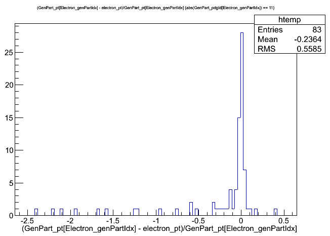
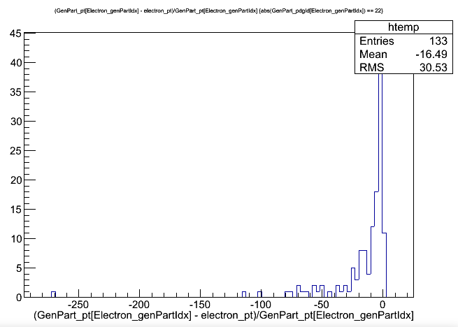
// Match electrons with gen particles and jets
for (auto p = selectedElectrons.begin(); p != selectedElectrons.end(); p++) {
 // Gen particle matching
 auto p4 = p->p4();
 auto idx = findBestVisibleMatch(interestingGenParticles, p4);
 if (idx != -1) {
   auto g = interestingGenParticles.begin() + idx;
   value_gen_pt[value_gen_n] = g->pt();
   value_gen_eta[value_gen_n] = g->eta();
   value_gen_phi[value_gen_n] = g->phi();
   value_gen_mass[value_gen_n] = g->mass();
   value_gen_pdgid[value_gen_n] = g->pdgId();
   value_gen_status[value_gen_n] = g->status();
   value_el_genpartidx[p - selectedElectrons.begin()] = value_gen_n;
   value_gen_n++;
 }

 // Jet matching
 value_el_jetidx[p - selectedElectrons.begin()] = findBestMatch(selectedJets, p4);
}

As an example of using these new branches, we can plot the electrons’ pT resolution and compare cases where the electrons were matched to a generated electron, vs where they were matched to a photon. Unsurprisingly, the resolution is much smaller for properly gen-matched electrons!

$ root -l output.root
[1] _file0->cd("aod2nanoaod")
[2] Events->Draw("(GenPart_pt[Electron_genPartIdx] - electron_pt)/GenPart_pt[Electron_genPartIdx]","abs(GenPart_pdgId[Electron_genPartIdx]) == 11");
[3] Events->Draw("(GenPart_pt[Electron_genPartIdx] - electron_pt)/GenPart_pt[Electron_genPartIdx]","abs(GenPart_pdgId[Electron_genPartIdx]) == 22");

Key Points

• Physics objects in CMS inherit common member functions for the 4-vector quantities of transverse momentum, polar/azimuthal angles, and mass/energy.

• Objects are matched to generator-level particles based on spatial relationships.

• Other quantities such as impact parameters and charge have common member functions.