Introduction

Overview

Teaching: 10 min
Exercises: 0 min

Questions

Why do we need data-driven background estimations? What is the ABCD method?

Objectives

Understand the motivation for data-driven background estimation

Get a first idea of the ABCD method

Background estimation methods

Estimating the event yields from different background processes, and the shape of these backgrounds as a function different variables, is a central task for any analysis. By data-driven background estimate, we mean an estimate that is essentially based on observed real collision events (data), although often these estimates also use some simulation-based information.

Data-driven estimates are useful to validate the predictions from simulations. Moreover, in some cases we know that our simulations cannot provide a reliable background estimate, and in these cases a data-driven background estimate is a must. Often this is the case with QCD multijet events. This is the background that we will estimate from data during this lesson.

In general, it is always desirable to rely on the observed events as much as possible, to minimize the risk that the results are incorrect due to some incorrect model or assumption used in the simulations. Over the decades countless background estimations have been developed, but here we will focus on one common method.

ABCD method

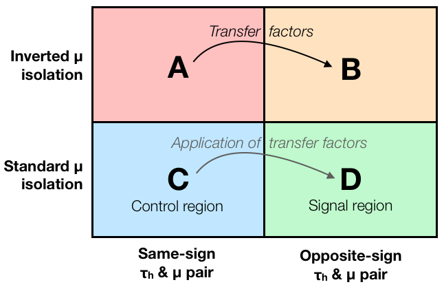
A common method to obtain a data-driven background estimate is the ABCD method. The idea of this method is illustrated in the diagram above.

To estimate a background process in our signal region D, a separate control region C is defined, and the background process is estimated in this region which is free of signal.

However, usually there can be some differences in the selection efficiency for the background process between regions C and D. To account for these differences, the estimate obtained in region C is corrected by so-called transfer factors. We will soon see how this all means in practice.

QCD estimation in Higgs to tau tau example

In this lesson, we will use the open data Higgs to tau tau analysis example](https://github.com/cms-opendata-analyses/HiggsTauTauNanoAODOutreachAnalysis), where the QCD multijet background is estimated with the ABCD method.

As shown in the diagram above, in this example the control region C is defined by selecting events with a same-sign tau pair (one hadronic tau and one muon from a tau decay), whereas the in the signal region D opposite-sign tau pair is required. The transfer factors are obtained from regions A and B, defined by inverting the isolation criterion used to select the muon.

Next we will see how to do all of this in practice. Here is one of the final output of the Higgs to tau tau analysis, (it is the di-tau mass, reconstructed from a hadronic tau candidate and a muon candidate) showing the different background processes including the QCD background estimate that we will produce during this lesson. All the other background are estimated from simulation in this analysis. Since this plot corresponds to tour signal region D, also the signal processes ggH and qqH are clearly visible in the plot.

Key Points

Data-driven background estimates are a must in situations where you cannot get a reliable estimate from simulation

They are also useful to validate predictions from simulations

The ABCD method is a common background estimated concept, based on four different regions in phase space

In this method, background shape in the signal region is estimated using a control region

Differences between the control region and signal region are accounted for by event weights called transfer factors

Control regions

Overview

Teaching: 10 min
Exercises: 10 min

Questions

What is a control region? How should we select our control region C?

Objectives

Understand the notions of signal and control regions

Learn the required features for a good control region

See how the control region is defined in Higgs to tau tau analysis example

Signal and control regions

By signal region, we mean the region in the phase space defined by our signal selection, i.e. the trigger and all offline selections that we use in the analysis.

In addition to signal region, often we need one or several control regions. These are usually obtained by changing some of the cuts w.r.t. our signal selection, to define regions that are in some aspects similar to signal region, but they are signal-depleted, i.e. the signal-to-background ratio is very tiny or even zero. Typically we want to define control regions that are enriched in a particular background process, and have sufficient statistics, i.e. there is enough events that enter the control region to give us sufficient statistical precision.

Sometimes control regions are also referred to as sidebands, especially in cases where the signal shows up as a resonance peak, so the signal region is defined by selecting some mass window, and the control regions are defined as sidebands on the left and right side of the mass window.

Signal and control regions in the ABCD method

In the ABCD method, region D is our signal region, whereas regions A, B and C are all control regions.

In the ABCD method, the region C is used to estimate the shape of the background process, as a function of one or several variables. Therefore we should aim to select a region where we can safely assume the background process to take similar shape as in the signal region D.

Next let us see what this means in the context of the Higgs to tau tau analysis.

Definition of control region C in the Higgs to tau tau analysis example

In the histograms.py script you can find the following lines:

        # Book histograms for the signal region
        df1 = df.Filter("q_1*q_2<0", "Require opposite charge for signal region")
        df1 = filterGenMatch(df1, label)
        hists = {}
        for variable in variables:
            hists[variable] = bookHistogram(df1, variable, ranges[variable])
        report1 = df1.Report()

        # Book histograms for the control region used to estimate the QCD contribution
        df2 = df.Filter("q_1*q_2>0", "Control region for QCD estimation")
        df2 = filterGenMatch(df2, label)
        hists_cr = {}
        for variable in variables:
            hists_cr[variable] = bookHistogram(df2, variable, ranges[variable])
        report2 = df2.Report()

As you can see, here define the signal regions by requiring that hadronic tau and the muon have opposite signs* (as they should if they are produced in a decay of a neutral Higgs boson), i.e. q_1*q_2<0, while the control region is defined by requiring them to have the same sign, i.e. q_1*q_2>0.

Challenge

Task: run the Higgs to tau tau analysis up to the step where you produce the histograms (python histograms.py) according to the instructions on this page.

Then inspect the histograms with ROOT TBrowser. Look at the histograms for the largest signal process (ggH), and compare the histograms showing the signal region (no postfix in the histogram name) and those showing the control region (_cr postfix in the histogram name). Which region has more signal?

The scroll through the selection of histograms to see all the different processes contained in this root file.

Estimating the QCD background in control region C

Often our control region C is not completely pure, so that it would contain only events produced by the background process we want to estimate. Instead, our data sample is a mixture of different processes. This is also the case in the Higgs to tau tau analysis example.

In order to estimate the yield and the shape of the QCD multijet background, we need to estimate all other processes that enter the control region, and subtract their contribution from the data. Luckily, we know how to estimate all the other relevant background processes – from simulation!

The subtraction of simulated processes (which are normalized to the integrated luminosity and the cross section), is done in the potting sxcript plot.py, where you can find the following lines:

    # Data-driven QCD estimation
    QCD = getHistogram(tfile, "dataRunB", variable, "_cr")
    QCDRunC = getHistogram(tfile, "dataRunC", variable, "_cr")
    QCD.Add(QCDRunC)
    for name in ["W1J", "W2J", "W3J", "TT", "ZLL", "ZTT"]:
        ss = getHistogram(tfile, name, variable, "_cr")
        QCD.Add(ss, -1.0)
    for i in range(1, QCD.GetNbinsX() + 1):
        if QCD.GetBinContent(i) < 0.0:
            QCD.SetBinContent(i, 0.0)

The point here is that this way, with the ABCD method, we can estimate the process that is difficult to simulate (QCD) by using data, as well as simulated samples for the background processes for which the simulations are relatively reliable (here: W+Jets, ttbar, Drell-Yan).

Soon we get to run this script and inspect the resulting QCD background estimate.

Key Points

Signal-depleted control regions are often used in background estimations

In the ABCD method, the background shape in signal region D is estimated using a control region C

To obtain estimate for a single process, e.g. QCD multijets, one can simply subtract other known (simulated) processes from data

Transfer factors

Overview

Teaching: 10 min
Exercises: 15 min

Questions

What is a transfer factor? How can we derive our transfer factors?

Objectives

Understand the concept of transfer factors, an their role in the ABCD method

See how the transfer factor is derived and applied in the in Higgs to tau tau analysis example

Transfer factors

Now that we know how to obtain our background shape from control region C, the next step is to figure out its proper normalization.

In practice it is impossible to find a control region where the selection efficiencies for each background process would be identical to the signal region. Even if the overall efficiency would be the same, probably the behavior is not identical as a function of all different variables considered in the analysis. Therefore we usually need to correct for the different selection efficiencies between regions C and D.

This correction is done by deriving additional event weights called transfer factors. In the simplest case, if we think that the background shape we get from region C is correct, we can just correct its normalization by scaling this background component by some factor – so our transfer factor is a single number, and we can weight all events in our background estimate by this single weight. However, usually also the transfer factor depends on one or several variables, so we need to apply different weights to different events.

The transfer factors are derived using two additional control regions, A and B (see the figure above). The idea is that the difference between A and B is defined by the same cut(s) as the difference between C and D, so if we parametrize the change of our background from A to B with transfer factors, these same factors should correctly describe the difference between C and D.

In case of a single transfer factor, we define it as a fraction of event yields: TF = N(B) / N(A). Then we can calculate the background yield in the signal region as N(D) = TF x N(C) = (N(B)/N(A)) x N(C). Another way to state is is that we assume that N(A)/N(B) = N(C)/N(D), and then the formula follows immediately. If we want to catch the dependence of transfer factors on different a variable, we can do this with histograms so that these same formulas hold for each single histogram bin. With multiple variables, we can use multi-dimensional histograms or just a set of one-dimensional histograms with varied selections so that we sample all the other variables that we want.

Application of a transfer factor in the Higgs to tau tau analysis example

In the Higgs to tau tau example, the transfer factor is applied in the plot.py script right after the lines we were already looking at:

    # Data-driven QCD estimation
    QCD = getHistogram(tfile, "dataRunB", variable, "_cr")
    QCDRunC = getHistogram(tfile, "dataRunC", variable, "_cr")
    QCD.Add(QCDRunC)
    for name in ["W1J", "W2J", "W3J", "TT", "ZLL", "ZTT"]:
        ss = getHistogram(tfile, name, variable, "_cr")
        QCD.Add(ss, -1.0)
    for i in range(1, QCD.GetNbinsX() + 1):
        if QCD.GetBinContent(i) < 0.0:
            QCD.SetBinContent(i, 0.0)
    QCDScaleFactor = 0.80
    QCD.Scale(QCDScaleFactor)

So here our transfer factor is a single number, 0.8, which is applied as an event weight to all events in our QCD histogram, effectively scaling the QCD background estimate down by 20 percent.

Challenge

Try changing the value of QCDScaleFactor e.g. to 0.5 or 1.0, re-run “python plot.py” and inspect how resulting plots change.

Derivation of a transfer factor in the Higgs to tau tau analysis example

At this point you might be wondering: where did this transfer factor come from? Let us find out by trying to derive it ourselves!

As discussed above, the code histograms.py produces the histograms for regions C and D. To derive transfer factors, we want to produce exactly the same histograms, but for regions A and B.

Let us define regions A and B so that they are identical to C and D, except that we invert the muon isolation criterion. Instead of requiring a tightly isolated muon (iso_1<0.1 ), let us use events with more loosely isolated muons and require ` iso_1>0.1` .

Challenge

Make a copy f the histograms.py file:
cp hisrograms.py histograms_antiiso.py
Then modify the file by changing the muon isolation cut from iso_1<0.1 to iso_1>0.1. Also change the output file name from histograms.root to histograms_antiiso.root. Then run the modified script to produce histograms for regions A and B:
python histograms_antiiso.py

Now that we have the histograms for regions A and B, we can use them to derive the transfer factors. For doing this, we use a separate script that is available here.

Challenge

Download the script transfer_factors.py to the same directory where you have your new histogram file histograms_antiiso.root, inspect what it does, and then run it:
wget https://raw.githubusercontent.com/cms-opendata-workshop/workshop-lesson-abcd-method/gh-pages/code/transfer_factors.py
python transfer_factors.py
What is the transfer factor given by the script?

(You should get a transfer factor of 1.09, which is actually quite different from 0.8 used in the original example. Our aim here is just to demonstrate the idea of transfer factor estimation.)

Key Points

Transfer factors are event weights that account for the differences between a control region and the signal region

In the ABCD method, they are derived by comparing regions A and B, and applied to transfer the background estimate from region C into the signal region D

Summary & discussion

Overview

Teaching: 10 min
Exercises: 0 min

Questions

What did we actually just do, and how realistic was it?

How is the ABCD method used in real life?

Objectives

Summarize what we have just learned

Get an idea of how ABCD method can be applied in more advanced ways

Summary of the ABCD method

By now, everything shown in this schematic should be clear to us, and we know how to do this in practice in Higgs to tau tau analysis.

Validation of the background estimate

But how can we convince ourselves that our background estimation method works and gives us a good estimate? One way to get some confidence is to define additional signal-free validation region, again by changing some cut(s) in the analysis, then split it into the four regions A, B, C, and D in the same way as in the original analysis, and check that the background estimate agrees with data. Then we know that the method works at least in the validation region. If we look at several validation regions “around” our signal region, we can gain even more confidence in our method.

Another common approach is to use pseudo-data, i.e. replace the real data with a sum of simulated samples, including the background we want to estimate with ABCD such as QCD. Then we can check that the background estimation method reproduces the correct results, because this time we know the “true” background composition of our pseudo-data. This simulated pseudo-data can also have some simulated signal included in the mix, so we can check that the signal doesn’t accidentally get absorbed into our background estimate.

Systematic uncertainties

Like all analysis steps, the ABCD method comes with some systematic uncertainties. Possible sources include (a) the systematic uncertainties of the simulated samples that are subtracted from data in regions A, B and C, (b) the statistical uncertainty of the background shape due to limited statistics in region C, (c) the statistical uncertainty of transfer factors due to limited statistics in regions A and B. In a realistic analysis, these (and possibly others) should be taken into account.

If the regions A, B, C and D are orthogonal, i.e. they do not contain same events, these different sources of uncertainty are independent, which makes them easier to handle in the statistical model used to extract the results (no worrying about correlations). Therefore in a typical analysis all signal and control regions are orthogonal (non-overlapping).

Often when choosing a suitable background estimation method (simulations, ABCD, something else..?), one needs to consider not only which methods give a reliable result, but also which method yields the smallest systematic and statistical uncertainty for the final result.

More advanced versions of the ABCD method

There are plenty of more advanced methods based on the simple ABCD idea. These can include analytic fits of distributions (to trade statistical uncertainties with possibly smaller fit uncertainties), sampling of the background shape and transfer factors in multiple dimensions (i.e. as a function of several different variables), simultaneous fits of all regions as well as possibly other control regions, etc. It has been shown that [using machine learning tools to optimize the selections] (https://arxiv.org/abs/2007.14400) for different regions can lead to further improvement in analysis sensitivity. So we have really just scratched the surface here, but now you have the basic knowledge to dive deeper when you feel like doing it!

Key Points

The basic concept of ABCD method is rather simple, but in practice things can get complicated

Careful validation of your background estimates is a necessity

There are several more advanced techniques in use, based on the basic concept of the ABCD method

Background estimation with the ABCD method

Introduction

Overview

Background estimation methods

ABCD method

QCD estimation in Higgs to tau tau example

Key Points

Control regions

Overview

Signal and control regions

Signal and control regions in the ABCD method

Definition of control region C in the Higgs to tau tau analysis example

Challenge

Estimating the QCD background in control region C

Key Points

Transfer factors

Overview

Transfer factors

Application of a transfer factor in the Higgs to tau tau analysis example

Challenge

Derivation of a transfer factor in the Higgs to tau tau analysis example

Challenge

Challenge

Key Points

Summary & discussion

Overview

Summary of the ABCD method

Validation of the background estimate

Systematic uncertainties

More advanced versions of the ABCD method

Key Points