Summary & discussion

Overview

Teaching: 10 min
Exercises: 0 min

Questions

• What did we actually just do, and how realistic was it?

• How is the ABCD method used in real life?

Objectives

• Summarize what we have just learned

• Get an idea of how ABCD method can be applied in more advanced ways

Summary of the ABCD method

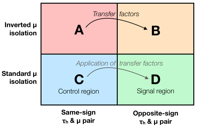
By now, everything shown in this schematic should be clear to us, and we know how to do this in practice in Higgs to tau tau analysis.

Validation of the background estimate

But how can we convince ourselves that our background estimation method works and gives us a good estimate? One way to get some confidence is to define additional signal-free validation region, again by changing some cut(s) in the analysis, then split it into the four regions A, B, C, and D in the same way as in the original analysis, and check that the background estimate agrees with data. Then we know that the method works at least in the validation region. If we look at several validation regions “around” our signal region, we can gain even more confidence in our method.

Another common approach is to use pseudo-data, i.e. replace the real data with a sum of simulated samples, including the background we want to estimate with ABCD such as QCD. Then we can check that the background estimation method reproduces the correct results, because this time we know the “true” background composition of our pseudo-data. This simulated pseudo-data can also have some simulated signal included in the mix, so we can check that the signal doesn’t accidentally get absorbed into our background estimate.

Systematic uncertainties

Like all analysis steps, the ABCD method comes with some systematic uncertainties. Possible sources include (a) the systematic uncertainties of the simulated samples that are subtracted from data in regions A, B and C, (b) the statistical uncertainty of the background shape due to limited statistics in region C, (c) the statistical uncertainty of transfer factors due to limited statistics in regions A and B. In a realistic analysis, these (and possibly others) should be taken into account.

If the regions A, B, C and D are orthogonal, i.e. they do not contain same events, these different sources of uncertainty are independent, which makes them easier to handle in the statistical model used to extract the results (no worrying about correlations). Therefore in a typical analysis all signal and control regions are orthogonal (non-overlapping).

Often when choosing a suitable background estimation method (simulations, ABCD, something else..?), one needs to consider not only which methods give a reliable result, but also which method yields the smallest systematic and statistical uncertainty for the final result.

More advanced versions of the ABCD method

There are plenty of more advanced methods based on the simple ABCD idea. These can include analytic fits of distributions (to trade statistical uncertainties with possibly smaller fit uncertainties), sampling of the background shape and transfer factors in multiple dimensions (i.e. as a function of several different variables), simultaneous fits of all regions as well as possibly other control regions, etc. It has been shown that [using machine learning tools to optimize the selections] (https://arxiv.org/abs/2007.14400) for different regions can lead to further improvement in analysis sensitivity. So we have really just scratched the surface here, but now you have the basic knowledge to dive deeper when you feel like doing it!

Key Points

• The basic concept of ABCD method is rather simple, but in practice things can get complicated

• Careful validation of your background estimates is a necessity

• There are several more advanced techniques in use, based on the basic concept of the ABCD method