Finding and exploring a NanoAOD dataset

Last updated on 2026-07-14 | Edit this page

Estimated time: 35 minutes

Overview

Questions

How do we find a specific nanoAOD dataset on the CERN Open Data Portal?
How do we use cernopendata-client to get file locations for a dataset?
How do we explore the content of a nanoAOD simulation file?

Objectives

Find a specific NANOAOD simulation dataset using the CERN Open Data Portal search tools
Use cernopendata-client to retrieve file locations for a chosen dataset
Inspect the content of a NANOAOD file using python tools

Find and explore a nanoAOD dataset

Now that you know how to navigate the CERN Open Data Portal, use cernopendata-client, and know a bit about NANOAOD format, let’s apply those skills together in a concrete example. We’ll find and explore simulated Z’ events in which the Z’ decays to a top and antitop quark pair — a dataset we will use throughout the workshop.

Callout

A Z’ (“Z-prime”) is a hypothetical heavy gauge boson that could arise from extensions of the Standard Model. A review of searches for the Z’ can be found here.

Find the dataset

All data can be found via the CERN Open Data Portal. Let’s search for simulated Z’ datasets. Dataset naming in CMS can seem obscure, but we can start with a broad wildcard search for Zprime*:

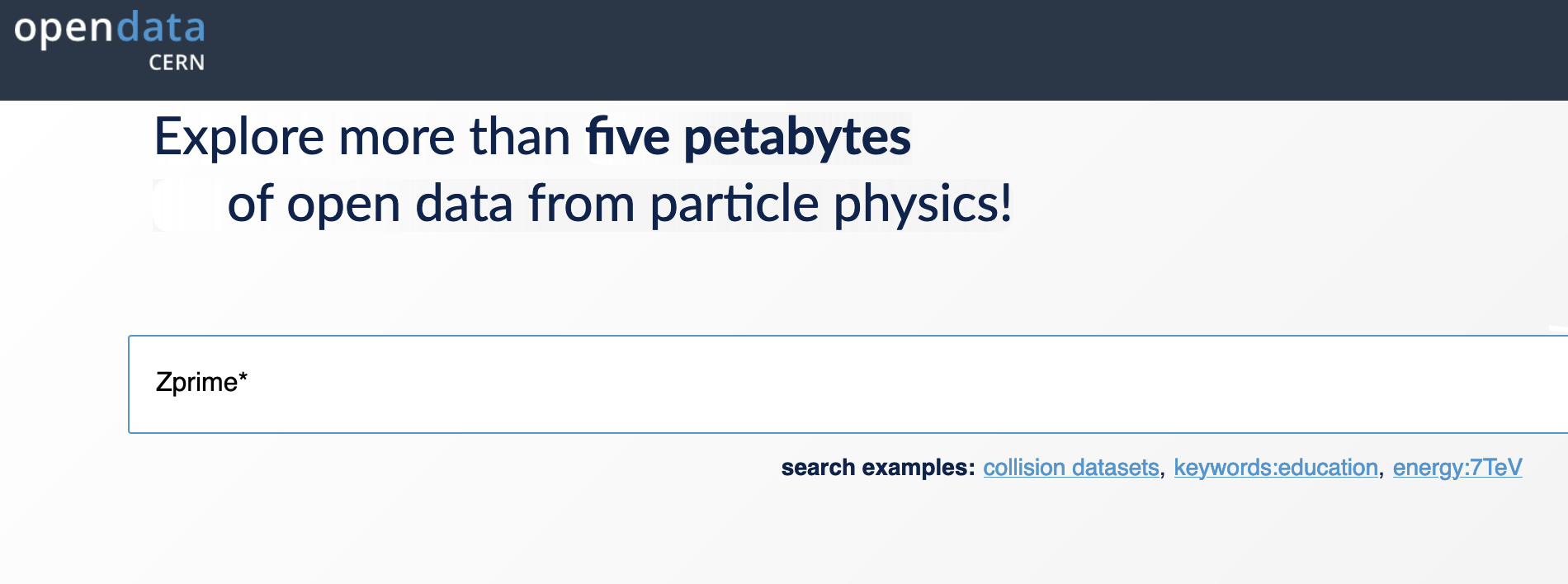
The query returns over 1000 records:

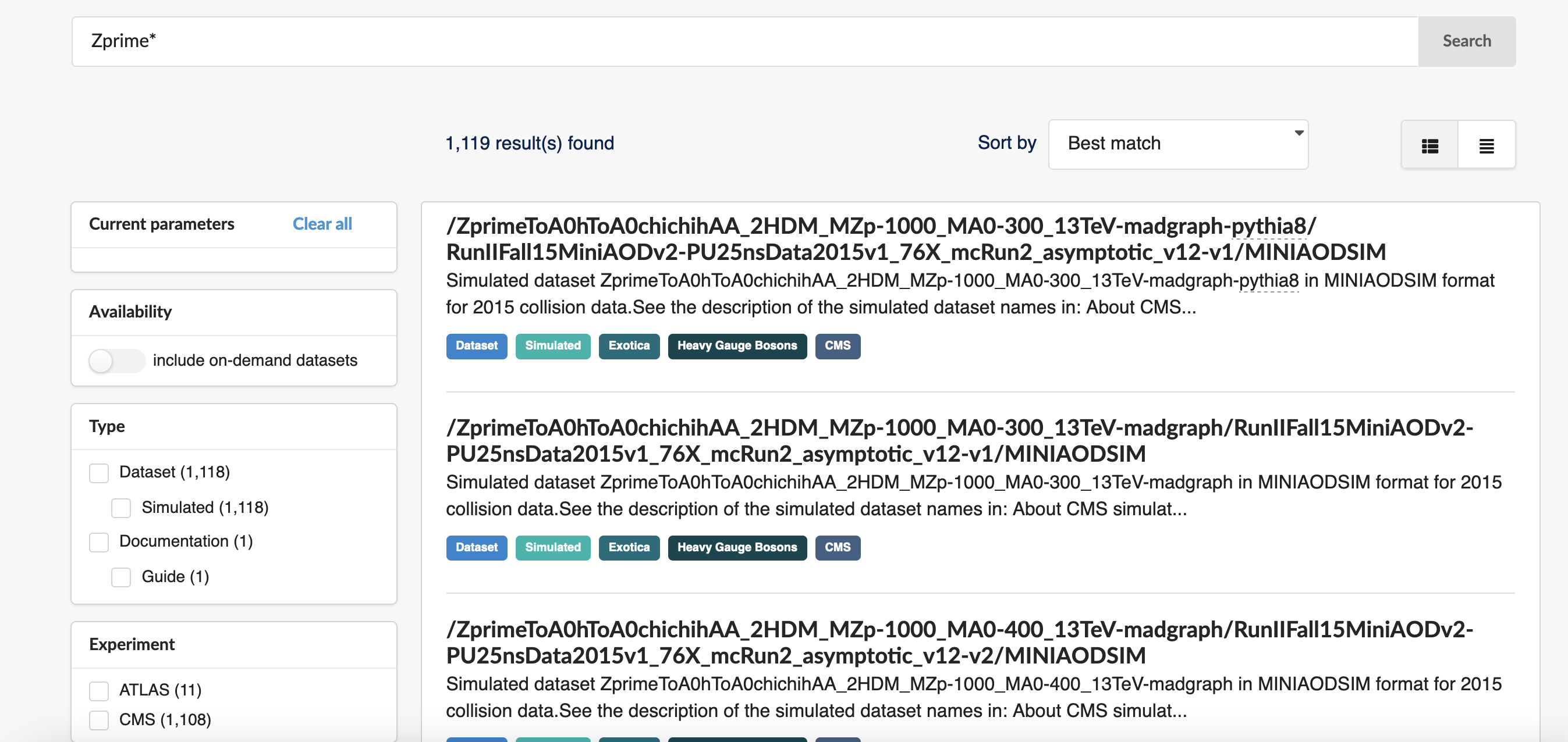
We can narrow the results by selecting Type: Dataset, Experiment: CMS, Year: 2016, File type: nanoaodsim, and Category: Heavy Gauge Bosons. This reduces the matches from over 1000 down to around 210:

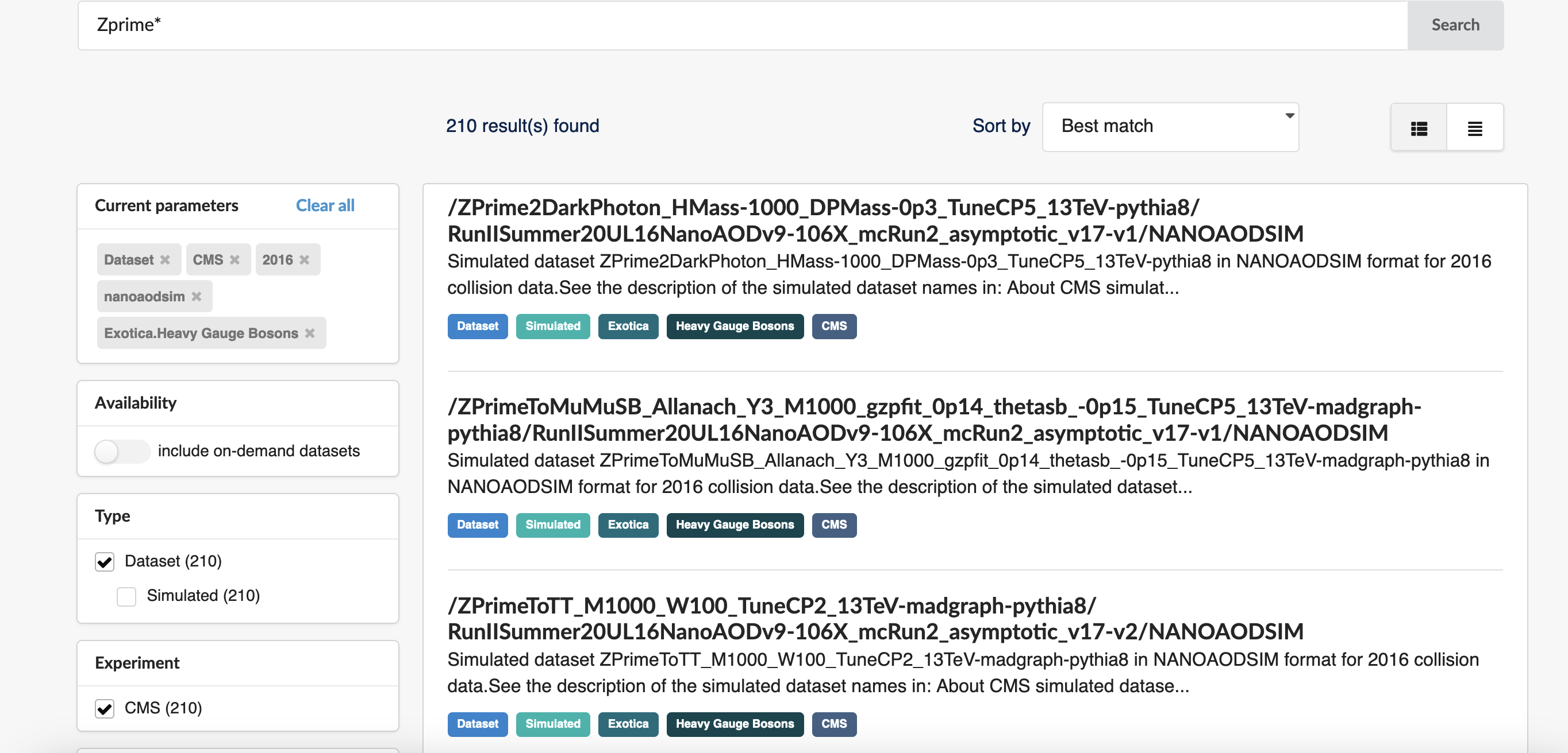
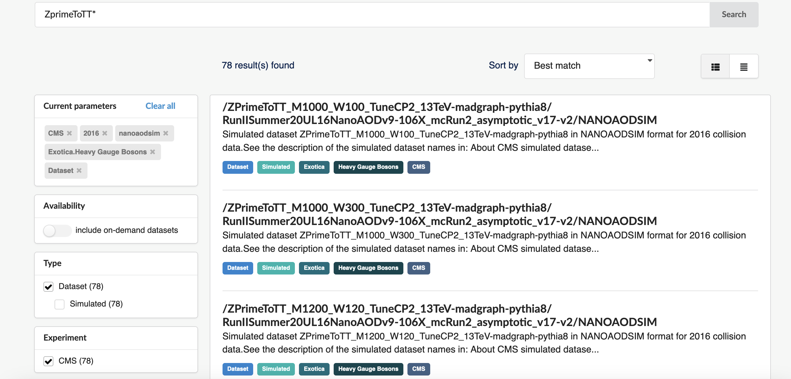
We can now read the dataset names more easily: “Zprime” is the particle produced, followed by its decay products. We want \(Z^{'} \rightarrow t\bar{t}\), which appears as “ZprimeToTT”. Let’s narrow further:

Dataset naming

The dataset names encode several pieces of information:

ZPrimeToTT — the particle produced and its decay (\(Z' \rightarrow t\bar{t}\))
M1000 — the mass (in GeV) of the hypothetical Z’ (here, 1000 GeV)
W100 — the width of the Z’ resonance (here, 100 GeV)
TuneCP2 — the underlying-event tune used in PYTHIA8
13TeV — the center-of-mass energy of the collision
madgraph-pythia8 — the event generators used (MadGraph for the hard process, PYTHIA8 for hadronization)

Several mass points are available in these results, spanning from 500 GeV to several TeV. The choice of mass point is part of your physics analysis strategy.

Exercises

Challenge

Exercise 1: Get data file locations

Choose a ZprimeToTT sample for a given mass and use cernopendata-client to retrieve the associated data file locations.

Recall what you’ve learned about cernopendata-client from Episode 4.

Show me the solution

Search for ZprimeToTT samples in the CERN Open Data Portal using the filters above. The resulting query is here.

Select a dataset. Here we use record 75124, “Simulated dataset ZPrimeToTT_M1000_W100_TuneCP2_13TeV-madgraph-pythia8 in NANOAODSIM format for 2016 collision data” (Z’ mass = 1000 GeV).

Confirm the available commands:

BASH

cernopendata-client --help

OUTPUT

Usage: cernopendata-client [OPTIONS] COMMAND [ARGS]...

  Command-line client for interacting with CERN Open Data portal.

Options:
  --help  Show this message and exit.

Commands:
  download-files      Download data files belonging to a record.
  get-file-locations  Get a list of data file locations of a record.
  get-metadata        Get metadata content of a record.
  list-directory      List contents of a EOSPUBLIC Open Data directory.
  verify-files        Verify downloaded data file integrity.
  version             Return cernopendata-client version.

Fetch the file locations for record 75124:

BASH

cernopendata-client get-file-locations --recid 75124

OUTPUT

http://opendata.cern.ch/eos/opendata/cms/mc/RunIISummer20UL16NanoAODv9/ZPrimeToTT_M1000_W100_TuneCP2_13TeV-madgraph-pythia8/NANOAODSIM/106X_mcRun2_asymptotic_v17-v2/2520000/65A0736B-22F3-C94C-99AE-36717B28629C.root
http://opendata.cern.ch/eos/opendata/cms/mc/RunIISummer20UL16NanoAODv9/ZPrimeToTT_M1000_W100_TuneCP2_13TeV-madgraph-pythia8/NANOAODSIM/106X_mcRun2_asymptotic_v17-v2/2520000/6E508763-A12F-8846-A295-F39EE7DDAA52.root
http://opendata.cern.ch/eos/opendata/cms/mc/RunIISummer20UL16NanoAODv9/ZPrimeToTT_M1000_W100_TuneCP2_13TeV-madgraph-pythia8/NANOAODSIM/106X_mcRun2_asymptotic_v17-v2/2530000/7B2D5CD5-9CAE-C046-A9AB-50CE9D48B187.root
http://opendata.cern.ch/eos/opendata/cms/mc/RunIISummer20UL16NanoAODv9/ZPrimeToTT_M1000_W100_TuneCP2_13TeV-madgraph-pythia8/NANOAODSIM/106X_mcRun2_asymptotic_v17-v2/260000/1A50245D-8213-6340-8EA0-CB064EEC6AF3.root
http://opendata.cern.ch/eos/opendata/cms/mc/RunIISummer20UL16NanoAODv9/ZPrimeToTT_M1000_W100_TuneCP2_13TeV-madgraph-pythia8/NANOAODSIM/106X_mcRun2_asymptotic_v17-v2/270000/09FA6C37-21D6-7846-B3E1-F8086CBA0E9E.root
http://opendata.cern.ch/eos/opendata/cms/mc/RunIISummer20UL16NanoAODv9/ZPrimeToTT_M1000_W100_TuneCP2_13TeV-madgraph-pythia8/NANOAODSIM/106X_mcRun2_asymptotic_v17-v2/270000/3AAB5B1E-7169-9C4D-841C-CB2D6E40CBAE.root
http://opendata.cern.ch/eos/opendata/cms/mc/RunIISummer20UL16NanoAODv9/ZPrimeToTT_M1000_W100_TuneCP2_13TeV-madgraph-pythia8/NANOAODSIM/106X_mcRun2_asymptotic_v17-v2/270000/820C3EBC-0E1D-CE41-9418-FA1615123FC2.root
http://opendata.cern.ch/eos/opendata/cms/mc/RunIISummer20UL16NanoAODv9/ZPrimeToTT_M1000_W100_TuneCP2_13TeV-madgraph-pythia8/NANOAODSIM/106X_mcRun2_asymptotic_v17-v2/270000/CF54D079-349C-FB4F-B6E5-3D579D89EDE4.root
http://opendata.cern.ch/eos/opendata/cms/mc/RunIISummer20UL16NanoAODv9/ZPrimeToTT_M1000_W100_TuneCP2_13TeV-madgraph-pythia8/NANOAODSIM/106X_mcRun2_asymptotic_v17-v2/80000/E964C281-43FB-D349-A436-9A3FDA0BAA28.root

To save these to a file for use in later analysis steps:

BASH

cernopendata-client get-file-locations --recid 75124 --protocol xrootd > files-recid-75124.txt

Challenge

Exercise 2: Inspect the data file

Using the file locations from Exercise 1 and the python tools you learned about in Episode 5, open one of the Z’ simulation files and explore its contents. Launch Jupyter Lab:

BASH

jupyter-lab

What variables are available? How does the jet content compare to what you saw in the SingleMuon collision data file?

Show me the solution

Import the necessary libraries in a notebook cell:

PYTHON

import uproot
import matplotlib.pylab as plt
import awkward as ak
import numpy as np

Open one of the Z’ files using the XRootD path:

PYTHON

file = uproot.open("http://opendata.cern.ch/eos/opendata/cms/mc/RunIISummer20UL16NanoAODv9/ZPrimeToTT_M1000_W100_TuneCP2_13TeV-madgraph-pythia8/NANOAODSIM/106X_mcRun2_asymptotic_v17-v2/2520000/65A0736B-22F3-C94C-99AE-36717B28629C.root")

Check the top-level content blocks:

PYTHON

file.classnames()

OUTPUT

{'tag;1': 'TObjString',
 'Events;1': 'TTree',
 'LuminosityBlocks;1': 'TTree',
 'Runs;1': 'TTree',
 'MetaData;1': 'TTree',
 'ParameterSets;1': 'TTree'}

Get the Events tree and list its variables:

PYTHON

events = file['Events']
events.keys()

You will see the same variable structure as in the collision data, but with additional Monte Carlo fields such as GenPart_* (generator-level particles) and genWeight. Because this is a \(Z' \rightarrow t\bar{t}\) sample, the events contain many jets from the top quark decays. Fetch the AK4 jet transverse momentum:

PYTHON

jet_pt = events['Jet_pt'].array()

Plot the distribution:

PYTHON

plt.hist(ak.flatten(jet_pt), bins=100, range=(0, 500))
plt.xlabel('Jet $p_T$ [GeV]')
plt.ylabel('Entries')
plt.title('AK4 jet $p_T$ — ZPrimeToTT M1000')
plt.show()

Compare the number of jets per event to what you saw in the SingleMuon data:

PYTHON

import numpy as np
print(f"Mean jets per event: {np.mean(ak.num(jet_pt)):.1f}")

You should observe a higher jet multiplicity here than in a typical collision data event, consistent with the two top quarks each decaying to a W boson and a b quark, with the W bosons decaying further.

To see the generator-level top quarks, look at the GenPart_* variables. For example, inspect the PDG IDs of the generated particles:

PYTHON

genpart_pdgid = events['GenPart_pdgId'].array()
print(genpart_pdgid[:3])

A PDG ID of 6 corresponds to a top quark and -6 to an antitop quark.

Key Points

Use the CERN Open Data Portal search filters (experiment, year, file type, category) to efficiently locate specific simulation datasets.
Dataset names encode the physics process, particle mass and width, collision energy, and generator software.
cernopendata-client retrieves file locations programmatically, making it easy to script dataset access.
NANOAODSIM files contain the same reconstructed-object variables as collision NANOAOD files, plus generator-level information such as GenPart_* and genWeight.