
The Complete Code
Last updated on 2026-07-24 | Edit this page
Estimated time: 10 minutes
Overview
Questions
- What does the finished MiniParT pipeline look like, before we build it piece by piece?
- Where can you find the complete pipeline as one unbroken block of code, without the surrounding explanation?
Objectives
- See the whole MiniParT pipeline once, as a map for the episodes that follow.
- Know where to find this code again later, for reference or for copying into a single notebook.
Before building this piece by piece, here’s the complete pipeline: reading raw CMS files, matching jets to their true Higgs-decay parents, training a transformer, and evaluating it. Don’t worry about following every line. The episodes that follow unpack each part, one at a time.
Step 1: Imports and feature list
PYTHON
import uproot
import awkward as ak
import vector
import numpy as np
import torch
import torch.nn as nn
from torch.utils.data import TensorDataset, DataLoader
from sklearn.model_selection import train_test_split
from sklearn.preprocessing import StandardScaler

vector.register_awkward()

# We avoid DeepJet/DeepCSV variables as requested.
# Using kinematics + energy fractions + pileup/multiplicity info.
FEATURE_NAMES = [
    'Jet_pt', 'Jet_eta', 'Jet_phi', 'Jet_mass',
    'Jet_chHEF', 'Jet_neHEF', 'Jet_chEmEF', 'Jet_neEmEF',
    'Jet_nConstituents', 'Jet_puId'
]

# Labels: 0 = Hbb, 1 = Hcc, 2 = QCD

# Streaming paths for the three validated CMS Open Data files this lesson
# uses (see "Working in Google Colab" for how these were confirmed).
TTHTOBB_PATH = "root://eospublic.cern.ch//eos/opendata/cms/mc/RunIISummer20UL16NanoAODv9/ttHTobb_M125_TuneCP5_13TeV-powheg-pythia8/NANOAODSIM/106X_mcRun2_asymptotic_v17-v2/260000/410F948C-6956-2D45-A170-DE6431E02281.root"

TTHTOCC_PATH = "root://eospublic.cern.ch//eos/opendata/cms/mc/RunIISummer20UL16NanoAODv9/ttHTocc_M125_TuneCP5_13TeV-powheg-pythia8/NANOAODSIM/106X_mcRun2_asymptotic_v17-v1/50000/5C12D3AA-9311-B840-BB5D-4155D7FF66E4.root"

QCD_BCTOE_PATH = "root://eospublic.cern.ch//eos/opendata/cms/mc/RunIISummer20UL16NanoAODv9/QCD_Pt_80to170_bcToE_TuneCP5_13TeV_pythia8/NANOAODSIM/106X_mcRun2_asymptotic_v17-v2/270000/A133135A-C83E-D245-846F-210C7AD2D29C.root"
Step 2: Extracting features and matching truth labels
PYTHON
def delta_phi(phi1, phi2):
    dphi = phi1 - phi2
    return (dphi + np.pi) % (2*np.pi) - np.pi

def extract_features(filepath, label, is_signal=True, max_events=None):
    tree = uproot.open(filepath)["Events"]

    # Load required branches
    branches = FEATURE_NAMES.copy()
    if is_signal:
        branches += [
            "GenPart_pdgId", "GenPart_pt", "GenPart_eta",
            "GenPart_phi", "GenPart_mass", "GenPart_genPartIdxMother"
        ]

    events = tree.arrays(branches, entry_stop=max_events)

    if is_signal:
        # Determine target quark based on label (0: b-quark=5, 1: c-quark=4)
        target_pdg = 5 if label == 0 else 4

        mother_idx = events.GenPart_genPartIdxMother
        valid = mother_idx >= 0
        mother_pdg = ak.where(valid, events.GenPart_pdgId[mother_idx], -999)

        is_higgs_dau = (abs(events.GenPart_pdgId) == target_pdg) & (mother_pdg == 25)
        mask = ak.num(events.GenPart_pt[is_higgs_dau]) == 2
        events = events[mask]
        is_higgs_dau = is_higgs_dau[mask]

        # Build 4-vectors
        jets = ak.zip({
            "pt": events.Jet_pt, "eta": events.Jet_eta,
            "phi": events.Jet_phi, "mass": events.Jet_mass
        }, with_name="Momentum4D")

        dau = ak.zip({
            "pt": events.GenPart_pt[is_higgs_dau], "eta": events.GenPart_eta[is_higgs_dau],
            "phi": events.GenPart_phi[is_higgs_dau], "mass": events.GenPart_mass[is_higgs_dau]
        }, with_name="Momentum4D")

        d1, d2 = dau[:, 0], dau[:, 1]

        # Match using dR < 0.4
        dr1 = np.sqrt((jets.eta - d1.eta[:, None])**2 + delta_phi(jets.phi, d1.phi[:, None])**2)
        dr2 = np.sqrt((jets.eta - d2.eta[:, None])**2 + delta_phi(jets.phi, d2.phi[:, None])**2)
        matched = (dr1 < 0.4) | (dr2 < 0.4)

        # Extract features for matched jets
        matched_events = events[matched]

        # Keep exactly 2 matched jets
        mask_2jets = ak.num(matched_events.Jet_pt) == 2
        final_events = matched_events[mask_2jets]

    else:
        # For QCD, require at least 2 jets and take the top 2 leading jets
        mask_2jets = ak.num(events.Jet_pt) >= 2
        events = events[mask_2jets]
        # Slice to keep only the first 2 jets
        final_events = events[:, :2]

    # Stack features into a NumPy array of shape (N_events, 2_jets, N_features)
    feature_list = []
    for feat in FEATURE_NAMES:
        # Fill missing values with 0 (e.g., puId might have NaNs depending on pt)
        arr = ak.fill_none(final_events[feat], 0)
        feature_list.append(ak.to_numpy(arr))

    X = np.stack(feature_list, axis=-1)
    y = np.full(X.shape[0], label)

    print(f"Loaded label {label}: {X.shape[0]} events")
    return X, y
Step 3: Preparing the data
PYTHON
# Extract features (adjust max_events to None when ready for full training)
X_bb, y_bb = extract_features(TTHTOBB_PATH, label=0, is_signal=True, max_events=50000)
X_cc, y_cc = extract_features(TTHTOCC_PATH, label=1, is_signal=True, max_events=50000)
X_qcd, y_qcd = extract_features(QCD_BCTOE_PATH, label=2, is_signal=False, max_events=50000)

# Combine datasets
X = np.concatenate([X_bb, X_cc, X_qcd], axis=0)
y = np.concatenate([y_bb, y_cc, y_qcd], axis=0)

# Train/Test Split
X_train, X_test, y_train, y_test = train_test_split(X, y, test_size=0.2, random_state=42, stratify=y)

# Normalize features (Transformers are sensitive to scale)
# We flatten to (N*2, Features) to fit the scaler, then reshape back
scaler = StandardScaler()
X_train_flat = X_train.reshape(-1, len(FEATURE_NAMES))
X_test_flat = X_test.reshape(-1, len(FEATURE_NAMES))

X_train_scaled = scaler.fit_transform(X_train_flat).reshape(-1, 2, len(FEATURE_NAMES))
X_test_scaled = scaler.transform(X_test_flat).reshape(-1, 2, len(FEATURE_NAMES))

# Convert to PyTorch tensors
train_data = TensorDataset(torch.tensor(X_train_scaled, dtype=torch.float32), torch.tensor(y_train, dtype=torch.long))
test_data = TensorDataset(torch.tensor(X_test_scaled, dtype=torch.float32), torch.tensor(y_test, dtype=torch.long))

train_loader = DataLoader(train_data, batch_size=256, shuffle=True)
test_loader = DataLoader(test_data, batch_size=256, shuffle=False)
OUTPUT
Loaded label 0: 36025 events
Loaded label 1: 37295 events
Loaded label 2: 50000 events
(Approximate - the exact counts depend on the files read, but land in this ballpark; see Preparing the Data.)
Step 4: Building MiniParT
PYTHON
class MiniParT(nn.Module):
    def __init__(self, input_dim, embed_dim=64, num_heads=4, hidden_dim=128, num_classes=3):
        super(MiniParT, self).__init__()

        # 1. Linear projection (Embedding)
        self.embedding = nn.Linear(input_dim, embed_dim)

        # 2. Transformer Encoder Layer (Self-Attention)
        encoder_layer = nn.TransformerEncoderLayer(
            d_model=embed_dim,
            nhead=num_heads,
            dim_feedforward=hidden_dim,
            batch_first=True,
            dropout=0.1
        )
        # Using just 2 layers for a "mini" model to keep local training fast
        self.transformer = nn.TransformerEncoder(encoder_layer, num_layers=2)

        # 3. Classification Head
        self.mlp = nn.Sequential(
            nn.Linear(embed_dim, hidden_dim),
            nn.ReLU(),
            nn.Dropout(0.1),
            nn.Linear(hidden_dim, num_classes)
        )

    def forward(self, x):
        # x shape: (Batch, Seq_Len=2, Features)

        # Project features
        x = self.embedding(x) # shape: (Batch, 2, embed_dim)

        # Apply self-attention
        x = self.transformer(x) # shape: (Batch, 2, embed_dim)

        # Mean pooling over the sequence (the 2 jets)
        x_pooled = x.mean(dim=1) # shape: (Batch, embed_dim)

        # Classify
        out = self.mlp(x_pooled) # shape: (Batch, num_classes)
        return out

torch.manual_seed(42)
np.random.seed(42)

model = MiniParT(input_dim=len(FEATURE_NAMES))
print(model)
OUTPUT
MiniParT(
  (embedding): Linear(in_features=10, out_features=64, bias=True)
  (transformer): TransformerEncoder(
    (layers): ModuleList(
      (0-1): 2 x TransformerEncoderLayer(
        (self_attn): MultiheadAttention(
          (out_proj): NonDynamicallyQuantizableLinear(in_features=64, out_features=64, bias=True)
        )
        (linear1): Linear(in_features=64, out_features=128, bias=True)
        (dropout): Dropout(p=0.1, inplace=False)
        (linear2): Linear(in_features=128, out_features=64, bias=True)
        (norm1): LayerNorm((64,), eps=1e-05, elementwise_affine=True)
        (norm2): LayerNorm((64,), eps=1e-05, elementwise_affine=True)
        (dropout1): Dropout(p=0.1, inplace=False)
        (dropout2): Dropout(p=0.1, inplace=False)
      )
    )
  )
  (mlp): Sequential(
    (0): Linear(in_features=64, out_features=128, bias=True)
    (1): ReLU()
    (2): Dropout(p=0.1, inplace=False)
    (3): Linear(in_features=128, out_features=3, bias=True)
  )
)
(Exact formatting can vary slightly by PyTorch version.)
Step 5: Training
PYTHON
device = torch.device("cuda" if torch.cuda.is_available() else "cpu")
model = model.to(device)

criterion = nn.CrossEntropyLoss()
optimizer = torch.optim.AdamW(model.parameters(), lr=1e-3, weight_decay=1e-4)

epochs = 10

for epoch in range(epochs):
    model.train()
    total_loss = 0
    correct = 0
    total = 0

    for batch_x, batch_y in train_loader:
        batch_x, batch_y = batch_x.to(device), batch_y.to(device)

        optimizer.zero_grad()
        outputs = model(batch_x)
        loss = criterion(outputs, batch_y)

        loss.backward()
        optimizer.step()

        total_loss += loss.item()
        _, predicted = outputs.max(1)
        total += batch_y.size(0)
        correct += predicted.eq(batch_y).sum().item()

    train_acc = 100. * correct / total
    print(f"Epoch {epoch+1}/{epochs} | Loss: {total_loss/len(train_loader):.4f} | Train Acc: {train_acc:.2f}%")
OUTPUT
Epoch 1/10 | Loss: 0.6823 | Train Acc: 65.98%
Epoch 2/10 | Loss: 0.6512 | Train Acc: 67.42%
Epoch 3/10 | Loss: 0.6301 | Train Acc: 68.55%
Epoch 4/10 | Loss: 0.6147 | Train Acc: 69.31%
Epoch 5/10 | Loss: 0.6029 | Train Acc: 69.98%
Epoch 6/10 | Loss: 0.5934 | Train Acc: 70.52%
Epoch 7/10 | Loss: 0.5856 | Train Acc: 70.94%
Epoch 8/10 | Loss: 0.5790 | Train Acc: 71.28%
Epoch 9/10 | Loss: 0.5734 | Train Acc: 71.58%
Epoch 10/10 | Loss: 0.5687 | Train Acc: 71.84%
(Illustrative - your own run will vary, but lands in the same ~0.68→0.56 loss, ~66%→72% accuracy range you’ll see explained in Training the Model.)
Step 6: Test accuracy
PYTHON
model.eval()
correct = 0
total = 0

# Store predictions for a confusion matrix if you want to plot one later
all_preds = []
all_labels = []

with torch.no_grad():
    for batch_x, batch_y in test_loader:
        batch_x, batch_y = batch_x.to(device), batch_y.to(device)

        outputs = model(batch_x)
        _, predicted = outputs.max(1)

        total += batch_y.size(0)
        correct += predicted.eq(batch_y).sum().item()

        all_preds.extend(predicted.cpu().numpy())
        all_labels.extend(batch_y.cpu().numpy())

test_acc = 100. * correct / total
print(f"Final Test Accuracy: {test_acc:.2f}%")
OUTPUT
Final Test Accuracy: 72.54%A typical run prints a final test accuracy around 71% (varies slightly run to run).
Step 7: Confusion matrix
PYTHON
import matplotlib.pyplot as plt
import seaborn as sns
from sklearn.metrics import confusion_matrix, roc_curve, auc
from sklearn.preprocessing import label_binarize
import torch.nn.functional as F

model.eval()

all_labels = []
all_preds = []
all_probs = []

with torch.no_grad():
    for batch_x, batch_y in test_loader:
        batch_x, batch_y = batch_x.to(device), batch_y.to(device)

        outputs = model(batch_x)

        # Apply softmax to get probabilities across the 3 classes
        probs = F.softmax(outputs, dim=1)
        _, predicted = outputs.max(1)

        all_probs.extend(probs.cpu().numpy())
        all_preds.extend(predicted.cpu().numpy())
        all_labels.extend(batch_y.cpu().numpy())

# Convert lists to NumPy arrays for easier slicing
all_labels = np.array(all_labels)
all_preds = np.array(all_preds)
all_probs = np.array(all_probs)

# Generate the matrix
cm = confusion_matrix(all_labels, all_preds)

# Plotting
plt.figure(figsize=(8, 6))
sns.heatmap(cm, annot=True, fmt='d', cmap='Blues',
            xticklabels=['Hbb (0)', 'Hcc (1)', 'QCD (2)'],
            yticklabels=['Hbb (0)', 'Hcc (1)', 'QCD (2)'])

plt.xlabel('Predicted Class', fontsize=12, fontweight='bold')
plt.ylabel('True Class', fontsize=12, fontweight='bold')
plt.title('miniParT Confusion Matrix', fontsize=14)
plt.show()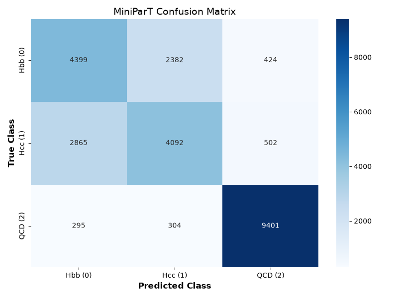
A typical run’s confusion matrix shows true Hcc events predicted as Hbb more often than correctly identified as Hcc, while QCD stays almost perfectly separated from both signal classes - see Evaluating the Model for a worked example with real numbers, and The Big Picture for how to read a confusion matrix.
Step 8: ROC curves
PYTHON
# Binarize the labels for One-vs-Rest ROC computation
# This turns a label like '1' into [0, 1, 0]
y_test_bin = label_binarize(all_labels, classes=[0, 1, 2])
n_classes = y_test_bin.shape[1]

plt.figure(figsize=(10, 8))
colors = ['blue', 'red', 'green']
class_names = ['Hbb', 'Hcc', 'QCD']

# Calculate and plot ROC for each class
for i, color, name in zip(range(n_classes), colors, class_names):
    # fpr = False Positive Rate, tpr = True Positive Rate
    fpr, tpr, _ = roc_curve(y_test_bin[:, i], all_probs[:, i])
    roc_auc = auc(fpr, tpr)

    plt.plot(fpr, tpr, color=color, lw=2,
             label=f'{name} vs Rest (AUC = {roc_auc:.3f})')

# Plot the random guessing baseline
plt.plot([0, 1], [0, 1], 'k--', lw=2, label='Random Guessing')

plt.xlim([0.0, 1.0])
plt.ylim([0.0, 1.05])
plt.xlabel('False Positive Rate (Background Efficiency)', fontsize=12)
plt.ylabel('True Positive Rate (Signal Efficiency)', fontsize=12)
plt.title('miniParT ROC Curves', fontsize=14)
plt.legend(loc="lower right", fontsize=11)
plt.grid(alpha=0.3)
plt.show()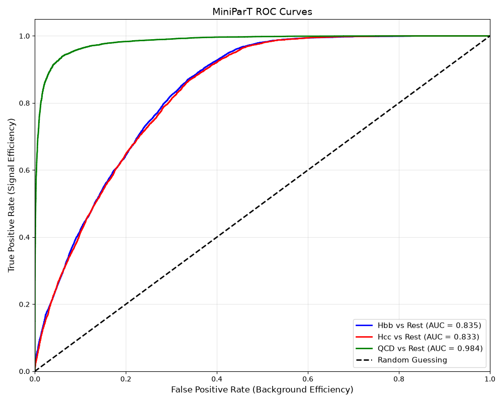
A typical run’s AUC values land around Hbb vs Rest ≈ 0.83, Hcc vs Rest ≈ 0.83, QCD vs Rest ≈ 0.98 - see The Big Picture for a refresher on what ROC curves and AUC measure.
Step 9: Fingerprint similarity
PYTHON
import torch.nn.functional as F
import pandas as pd

model.eval()

# 1. Define a helper function to bypass the final MLP and get the 64D vector
def get_fingerprint(event_tensor):
    with torch.no_grad():
        # Project into 64D
        emb = model.embedding(event_tensor)
        # Pass through Self-Attention
        contextualized = model.transformer(emb)
        # Pool to get the per-event 64D fingerprint
        fingerprint = contextualized.mean(dim=1)
    return fingerprint

# 2. Group every test event by its true class
hbb_events = torch.tensor(X_test_scaled[y_test == 0], dtype=torch.float32).to(device)
hcc_events = torch.tensor(X_test_scaled[y_test == 1], dtype=torch.float32).to(device)
qcd_events = torch.tensor(X_test_scaled[y_test == 2], dtype=torch.float32).to(device)

# 3. Fingerprint every event, then average within each class into one
# representative 64D vector per class (see the explanation below)
fp_hbb = get_fingerprint(hbb_events).mean(dim=0, keepdim=True)
fp_hcc = get_fingerprint(hcc_events).mean(dim=0, keepdim=True)
fp_qcd = get_fingerprint(qcd_events).mean(dim=0, keepdim=True)

# 4. Compute Cosine Similarities
# Cosine similarity bounds the dot product between -1 and 1
sim_hbb_hcc = F.cosine_similarity(fp_hbb, fp_hcc).item()
sim_hbb_qcd = F.cosine_similarity(fp_hbb, fp_qcd).item()
sim_hcc_qcd = F.cosine_similarity(fp_hcc, fp_qcd).item()

# 5. Display the results in a clean table
print("Cosine Similarity Matrix (1 = Identical, -1 = Opposite):\n")

data = {
    "Hbb": [1.0, sim_hbb_hcc, sim_hbb_qcd],
    "Hcc": [sim_hbb_hcc, 1.0, sim_hcc_qcd],
    "QCD": [sim_hbb_qcd, sim_hcc_qcd, 1.0]
}

df_sim = pd.DataFrame(data, index=["Hbb", "Hcc", "QCD"])
print(df_sim.round(3))
OUTPUT
Cosine Similarity Matrix (1 = Identical, -1 = Opposite):

        Hbb    Hcc    QCD
Hbb   1.000  0.712 -0.183
Hcc   0.712  1.000 -0.146
QCD  -0.183 -0.146  1.000
(Approximate - depends on the actual training run.)
This compares the average fingerprint across every test event in each class, not one event per class. Comparing single events instead is unreliable enough to look actively backwards: in one single-event comparison, Hbb and Hcc came out with cosine similarity -0.057 (opposite directions) despite being the two classes the model confuses constantly, while Hbb and QCD came out at +0.322 (similar direction) despite QCD being the class the model separates most cleanly (AUC ≈ 0.98). Neither number reflects what the model actually learned - both are noise from picking one arbitrary event per class. Averaging over every test event in a class cancels that noise out, leaving a genuinely representative direction for what the model learned about that class as a whole. See The Big Picture for what cosine similarity measures in the first place.
- This episode previews the complete pipeline, from reading raw CMS files to plotting results, with minimal explanation beyond notes on typical output.
- The episodes that follow build the same pipeline piece by piece, covering the physics and the code behind each part.