The Big Picture
Last updated on 2026-07-24 | Edit this page
Estimated time: 20 minutes
Overview
Questions
- What physical process are we trying to classify when we look at a pair of jets from the CMS detector?
- Why is telling Hbb and Hcc jets apart harder than telling either of them apart from QCD background?
- Why does this problem call for machine learning instead of a hand-written rule?
- What does “mini” mean in MiniParT, and how does it relate to the full-scale Particle Transformer used in real CMS analyses?
Objectives
- Describe the physics goal of this lesson: classifying jet pairs as Hbb, Hcc, or QCD background.
- Explain why bottom-quark and charm-quark jets are hard to tell apart.
- Describe what “training” a model means, and why simulated data is needed to do it.
- Explain why a transformer architecture is used here, and what “mini” simplifies compared to the full-size version.
The question we’re trying to answer
Deep inside the CMS detector at CERN, protons collide at nearly the speed of light. (For background on the detector itself - its layers, subsystems, and how it records a collision - see the CMS Open Data Workshop’s detector lesson; this lesson picks up from there.) Occasionally, a collision briefly creates a Higgs boson - a heavy, short-lived particle that almost instantly decays into other particles. We care about three outcomes:
- The Higgs decays into two bottom quarks (“Hbb”).
- The Higgs decays into two charm quarks (“Hcc”).
- Nothing to do with a Higgs boson at all - just ordinary background, called “QCD.”
Quarks can’t fly around on their own: as they shoot away from the collision, they drag along a spray of other particles, called a jet. So what we actually see in the detector is jets, not quarks.
Our job: look at a pair of jets and guess whether they came from Hbb, Hcc, or QCD.
This is hard because bottom and charm quarks are cousins - both “heavy” quarks that behave similarly when they turn into jets. Telling their jets apart is a genuinely open problem in particle physics; telling either of them apart from ordinary QCD jets is easier. Keep those as two separate questions as you go through this lesson (“is this a Higgs event at all?” vs. “Hbb or Hcc?”) - you’ll see the distinction again in the confusion matrix in the evaluation episode.
Why use AI for this at all?
A human physicist can’t look at raw detector data and just “see” whether a jet came from a bottom quark, a charm quark, or nothing special. But each jet leaves subtle clues - how its energy splits between charged and neutral particles, how spread out it is, how many particles it contains. No single clue is a smoking gun, but combined, they carry real information. That’s exactly the kind of problem machine learning is good at: finding a pattern across many weak, noisy clues that no simple rule can capture.
What is “machine learning,” in one paragraph?
Instead of a person writing rules like “if energy fraction > 0.6 then it’s probably a bottom quark,” we show a computer program thousands of examples where we already know the right answer (because the data is simulated - see Finding the Truth Labels), and let it gradually adjust itself until it gets good at guessing correctly. That process is “training,” and the program doing the adjusting is the “model.”
Why a transformer, and why “mini”?
A transformer is a model that’s very good at looking at a set of things and figuring out how they relate to each other - famously used for understanding sentences, and also used in real CMS analyses to look at a set of jets. We only have two jets per event here, so this is a toy-sized version of the same idea used in professional particle physics AI - hence MiniParT (“mini Particle Transformer”).
It’s “mini” because: - It only looks at 2 jets at a time (real versions can handle 100+ particles per jet) - It only uses 10 simple numbers per jet (real versions use many more) - It’s small enough to train on a laptop in minutes, not hours
MiniParT trades away detail (raw particle-level information, larger networks, more jets per event) in exchange for being small enough to fully understand and train quickly. Real CMS analyses use the full-size Particle Transformer specifically because that extra detail helps with the hard Hbb-vs-Hcc problem - nothing about “mini” changes the physics goal, only how much information the model has to work with.
Roadmap
This lesson runs entirely in Google Colab: the next episode sets that up and streams CMS data directly from CERN, and the one right after previews the complete MiniParT pipeline. It’s not something to copy into your notebook yet. From episode 4 on, the lesson builds MiniParT for real, step by step:
- Working in Google Colab - setting up Colab and streaming CMS Open Data directly, without downloading anything
- The Complete Code - a preview of the finished pipeline
- What Is a Jet? - the raw ingredients: 10 numbers per jet
- Finding the Truth Labels - how we know the “right answer” for training
- Preparing the Data - getting the numbers ready for a neural network
- Building MiniParT - the model itself, piece by piece
- Training the Model - how it actually learns
- Evaluating the Model - did it work, and how do we know?
Episodes 4 through 9 follow the same shape: each opens with the complete code for that episode, ready to run in one go, followed by a line inviting you to read on. Copy that opening block into a new cell, run it, and then read the prose that follows - that’s where the actual teaching happens, walking back through the code you just ran one small idea at a time: why a feature is included, what a line of PyTorch is really doing, why a step needs to happen before another one. Where a code block produces visible output (a print statement, a shape, a plot), a block right underneath it shows what you should see.
These opening code blocks are cumulative from episode 2 onward, and each assumes every earlier one is already in your notebook, run in order. Episode 3 is the exception. It’s a preview, not a building block, so skip pasting it in. By the end of episode 8, your notebook is a trained MiniParT model.
How we’ll judge whether it worked
Later in this lesson, in Evaluating the Model, we check whether MiniParT actually learned something useful, using three tools covered there in full: a confusion matrix, ROC curves with AUC, and comparing the model’s internal representations with cosine similarity. Here’s a short preview of the first two, using illustrative data, so you recognize them when you meet them for real.
Confusion matrix, in brief: a grid where rows are the true class and columns are the model’s guess, so a perfect model has large numbers only on the diagonal.
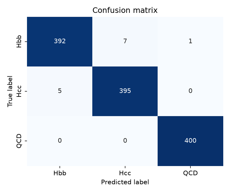
This example shows good overall performance - most events land on the diagonal - but look closely and there’s visible confusion between two of the three classes (a handful of events leak each way between them), while the third class is separated from both almost perfectly. That exact pattern, two classes that are hard to tell apart plus a third that isn’t, is the situation this lesson’s Hbb/Hcc/QCD problem is actually in.
(Both this example and the one below are generated with the same sklearn/seaborn/matplotlib code shown later in this lesson, using illustrative data, not this lesson’s actual results.)
ROC curve and AUC, in brief: a curve tracing the tradeoff between catching more real signal and letting more background through, as the model’s confidence threshold slides from strict to loose; AUC condenses that whole curve into one number from 0 to 1.
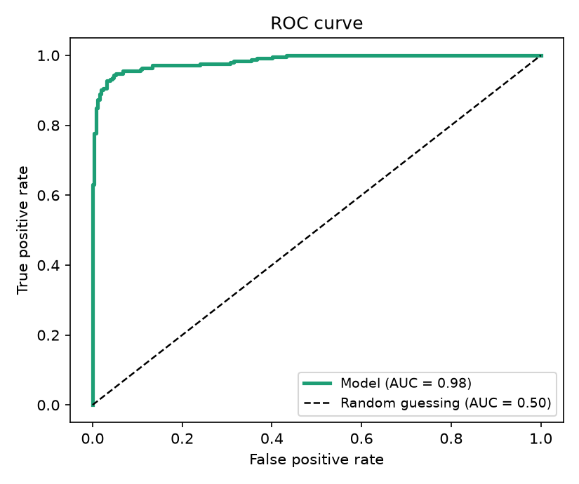
A curve that hugs the top-left corner, away from the diagonal, is what strong separation looks like - catching signal while letting almost no background through. AUC boils that shape down to a single number: close to 1.0 means close to that corner, close to 0.5 means close to the diagonal, no better than a coin flip. The AUC near 1 shown here is illustrative, not this lesson’s actual number.
Dot product / cosine similarity, in brief: the model represents every event internally as a vector of 64 numbers, and cosine similarity compares two such vectors by direction alone, ignoring length - close to 1 means pointing the same way, close to -1 means opposite, close to 0 means unrelated. Evaluating the Model uses this to sanity-check what the model learned internally, independent of its final guess.
Question
Q: A friend says “the model just needs to learn to recognize a Higgs boson in the data.” What is slightly wrong with that, and what is the model actually being asked to do?
A: The model never sees a Higgs boson directly - it decays before reaching the detector. The model sees two jets and has to guess, from 10 summary numbers per jet, whether that pair is more consistent with Hbb, Hcc, or QCD. “Recognizing a Higgs boson” really means recognizing patterns in the jets it leaves behind.
- We’re teaching a computer to classify pairs of jets into Hbb / Hcc / QCD.
- We use simulated CMS data because it comes with a built-in answer key.
- MiniParT is a scaled-down version of a real particle physics AI architecture - small enough to fully understand, built the same way the real ones are.