Modeling backgrounds in your analysis: All in One View

Content from What are backgrounds

Last updated on 2024-07-31 | Edit this page

Estimated time: 11 minutes

Overview

Questions

What do we mean when we say “backgrounds”?
Are all backgrounds the same?
What do we mean by “model backgrounds”?

Objectives

To develop an understanding of the terms, like background modeling

Introduction

As a reminder, we’re going to reproduce parts of a 2019 CMS study for resonant production of top-antitop pairs. The paper can be found here and hypothesizes a particle with specific properties referred to as $Z'$ which is produced in our proton-proton collisions and then decays to a top-antitop pair.

\[p p \rightarrow Z' \rightarrow t\overline{t}\]

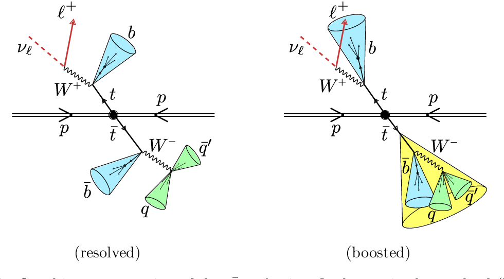
Two diagrams showing a top quark and antitop quark being produced where one decays through a leptonic process and the other decays through a hadronic process. The first image shows the hadronic decay in a non-boosted state and the second image shows the hadronic jets overlapping because of the boosted nature of the decay.

A challenge is that there are standard model processes than can produce the same final state objects and can mimic our signal. We have chosen selection criteria such that the kinematics are different from our signal, but we can’t entirely eliminate all the standard model processes and so we need to estimate how much of the remaining collision data can be explained by these background processes.

Backgrounds

In particle physics we are usually either a) searching for new physics or b) trying to make a precise measurement of some standard model process.

In the case of the former, we can almost never entirely get rid of all the standard model processes. In the case of the latter, we can almost never get rid of all the other standard model processes that are not the one we’re interested in. In both cases, these remaining data are referred to as backgrounds.

Backgrounds can come in different forms.

Standard model processes that produce the same final state as what we are interested in
Mistakes in how we reconstruct our physics objects such that it looks like we have the same final state

The first case is usually what we are dealing with at the LHC experiments.

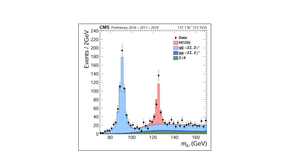
For example, let’s look at this plot showing a Higgs measurement (formerly a Higgs discovery!). This type of plot is ubiquitous in high energy physics analysis. It shows a stacked histogram of Monte Carlo (simulation) for the signal (Higgs) and background processes, compared with the collision data overlaid.

It is obvious that without the inclusion of the Higgs hypothesis we would not be able to fully describe these data.

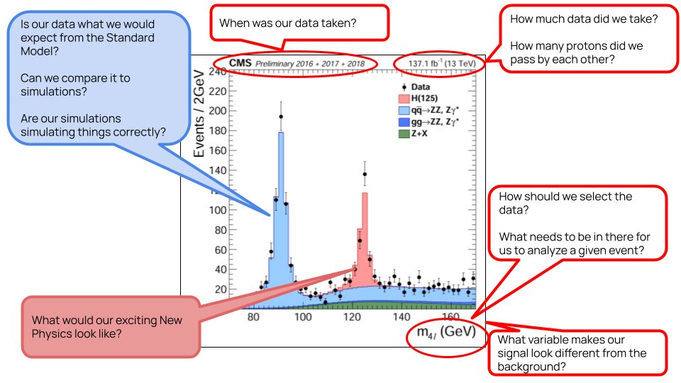
Plot of 4-lepton final state from CMS showing Higgs peak

Now let’s step back and take a look at everything that went into this plot! While we are not going to go through all of this, we draw your attention to the comments about the standard model processes: our backgrounds. Since we are working our way through an exercise where we search for signs of new physics, understanding our background contributions is incredibly important.

Plot of 4-lepton final state from CMS showing Higgs peak with some text describing what goes into this plot.

Background processes for our analysis

As a reminder, we will concern ourselves with four (4) physics processes that might mimic our signal and which we identify as possible backgrounds.

Production of a top-quark pair that decays semileptonically
Production of a top-quark pair that decays hadronically
Production of a top-quark pair that decays leptonically
Production of $W$ bosons in association with jets and when the $W$ bosons decay leptonically

We made some cuts on the data to reduce these contributions quite a bit, but we can’t get rid of them entirely.

For our analysis, we will use our simulations to estimate the amount that these contribute to the final dataset. But first, let’s walk through a simple example of data-driven background estimation.

Key Points

Backgrounds can manifest in your analysis for different reasons
It’s almost impossible to eliminate all backgrounds in collider experiments

Content from Data-driven background estimation

Last updated on 2024-07-31 | Edit this page

Estimated time: 22 minutes

Overview

Questions

Can we use the actual data to estimate backgrounds?
What are the downsides to this approach?

Objectives

Learn to use the simplest sideband approach to estimating backgrounds
Recognize how this might be extended to more complicated approaches

Introduction

There is a significant amount of code to run here and so we have written the majority of it in a Jupyter notebook. You can run most of the code on its own, but you should take the time to read and understand what is happening. In some places, you need to modify the code to get it to run.

First, start your python docker container, following the lessons from the pre-exercises. I am on a Linux machine, and I have already created the cms_open_data_python directory. So I will do the following

BASH

export workpath=$PWD
mkdir cms_open_data_python
chmod -R 777 cms_open_data_python

Start the container with

BASH

docker run -it --name my_python -P -p 8888:8888 -v ${workpath}/cms_open_data_python:/code gitlab-registry.cern.ch/cms-cloud/python-vnc:python3.10.5

You will get a container prompt similar this:

OUTPUT

cmsusr@4fa5ac484d6f:/code$

Before we start our Jupyter environment, let’s download the notebook we’ll be using with the following command.

BASH

wget https://raw.githubusercontent.com/cms-opendata-workshop/workshop2024-lesson-background-modeling/main/instructors/background_modeling_lesson.ipynb

Now I will start Jupyter lab as follows.

BASH

jupyter-lab --ip=0.0.0.0 --no-browser

and open the link that is printed out in the message.

How to follow this lesson

While some of the code will be explained on this web page, the majority of the code and explanations of the code are written out in the Jupyter notebook. Therefore, you should primarily following along there.

I will use this webpage for the lesson to provide guideposts and checkpoints that we can refer to as we work through the lesson.

Data-driven background estimation

Preparing the environment

We will be making use of the pandas and Hist python libraries.

Pandas
Hist

The first part of the notebook Install and upgrade libraries asks you to do just that, in order to ensure a consistent environment.

Depending on your connection, it should take less than 1 minute to upload and import the libraries.

Sideband estimation

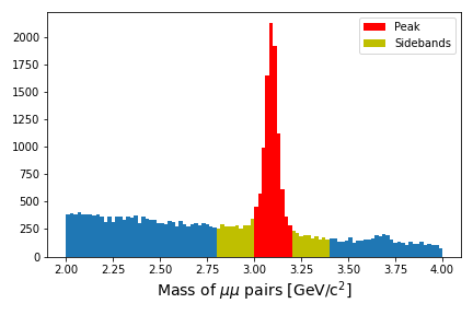
Suppose you are studying the production of $J/\psi$ mesons and you are able to reconstruct the invariant mass of muon pairs. Sometimes those muon pairs come from the decay of $J/\psi$ but they might come from any number of other processes.

You are not interested in exactly what those background processes are, you only want to know how many $J/\psi$ mesons are in your dataset.

There are sophisticated ways to fit the data distribution but we will do something simpler. We will estimate the amount of background events “under” the peak and then subtract that from the signal region to get an estimate of the number of events.

The figure below shows a graphical representation of the sidebands relative to your peak.

A plot of the invariant mass of muon pairs from CMS open data showing the $J\psi$ peak on a falling background.

Run through the notebook to walk through this exercise.

Can you do better?

The example in the notebook leads to an estimate of 7745.5 $J/\psi$ events in the dataset. However, the values we chose are maybe not perfectly centered on the peak. Does it matter? Can you play around with the definitions of the signal region or sideband region to come up with a different estimate.

Put your own estimates for the number of $J/\psi$ mesons in the Zoom chat or Mattermost discussion.

This simple sideband approach can be extended to something referred to as the ABCD which extends the sidebands into some 2-dimensional kinematic region.

Key Points

The simplest data-driven approach to background estimates is the sideband approach
This can be good enough for a first-order estimate when there is an obvious peak

Content from Simulation-based background estimation

Last updated on 2024-07-31 | Edit this page

Estimated time: 31 minutes

Overview

Questions

How can we use our simulation samples to estimate our background?
Can we use our simulation samples “as-is”?

Objectives

Learn to use simulation samples to estimate background
Understand how weights are used to compare data and simulation
Make a plot to compare our simulations of background samples to the collision data

Introduction

At the end of this lesson, you’ll have a plot similar to the Higgs plot at the start of this lesson, in which you compare the background and signal Monte Carlo to the collision data and try to determine if there is an obvious signal in the dataset.

You’ll be walking through the Jupyter notebook to do this, but first we want to introduce the idea of scaling your Monte Carlo and how generator weights come into play.

You can also read more about background estimation at the CMS Open Data Guide chapter on this topic

Cross sections

It is worth reminding ourselves of the meaning of cross sections and integrated luminosity.

Instantaneous luminosity is effectively a measure of how many protons pass close enough to the other proton bunches that they might interact in some time interval. You can think of it as the “brightness” of our beams.

Integrated luminosity ($\mathcal{L}$) is the sum of all of those potential interactions. Effectively, it refers to the amount of collected data.

Cross sections ($\sigma$) are related to the probability of a particular process, either production or decay, occurring.

From this, we can get the expected number of events $N$.

\[N = \sigma \times \mathcal{L}\]

Scaling Monte Carlo

We often overproduce our Monte Carlo so that we have more than there would be in data. This reduced the statistical uncertainty that might come from small samples after they are reduced by our selection cuts.

So if we want to compare our Monte Carlo simulation samples to the collision data, we need to know what the cross section is for those processes, We can calculate the expected number of events ($N_{exp}$) from the above equation and then scale our produced number of events ($N_{gen}$) to get the weight, for that dataset.

\[\textrm{weight} = \frac{N_{exp}}{N_{gen}}\] \[\textrm{weight} = \frac{\sigma \times \mathcal{L}}{N_{gen}}\]

Monte Carlo weights

When Monte Carlo events are generated, there is a weight associated with each event that is an output of the particular generator. Because you might want a lot of simulated events generated in a region of phase space that is normally sparsely populated, you need a way to effectively normalize the full simulated dataset.

Depening on the generator, you might sometimes get negative weights. When we scale everything, we count up the number of events with positive weight and subtract from it the number of events with negative weights. For the Monte Carlo samples we are using for this lesson, we have almost no events with negative weights, but it is good to know this for future analyses.

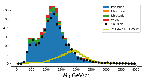
Final plot

If you are able to get through your Jupyter notebook, you should wind up with a plot that compares the simulation with the collision data.

It’s pretty good agreement, just from scaling things! For the next sections, you’ll learn how to use more sophisticated inference tools to estimate the upper-limit on the $Z'$ production cross section.

A plot of the ttbar invariant mass from our analysis with simulation and collision data labeled.

Key Points

Awkward arrays allow for a simplified syntax when making cuts to select the data
You need to be careful to distinguish between cuts on events and cuts on particles