What is reinterpretation and what is the role of open data?
Overview
Teaching: 20 min
Exercises: 0 minQuestions
What is reinterpretation?
What are exact and optimized reinterpretation?
What inputs are needed to perform reinterpretation?
What is the role of open data in reinterpretation?
Objectives
Learn the concepts of exact reinterpretation and optimized reinterpretation.
Learn the inputs needed to perform different types of reinterpretation.
Learn the role of open data in different types of reinterpretation.
What is reinterpretation?
LHC is building a tremendous physics legacy through the vastly many analyses performed by the experiments. CMS alone has published more than a thousand physics analyses. These analyses focus on a large spectrum of physics goals ranging from standard model measurements to searches for new physics. Each of these analyses investigate well-defined final states that characterize predicted signatures from a physics model or a set of physics models. The physicists who originally design and perform an analysis usually interpret the analysis result based on one or more physics models.
Experimental result vs. interpretation
Results and interpretation are two terms that are sometimes used interchangeably, even though they refer to two very distinct concepts. Let us first clarify those:
- An experimental result is the empirical outcome of the experiment, the measurement of some physical quantity, such as counts, cross sections, signal strengths, masses, etc.
- Interpretation is the comparison of experimental results with the expectations of a given a theoretical model. We use a statistical model that relates to observed quantities in data (e.g.. counts) to the theoretical model parameters (e.g. BSM particle masses, cross sectons). Take the simplest case of a counting experiment with observes data counts D and estimated background B after the analysis selection: interpretation first calculates the signal counts S predicted by the model after the analysis selection, then checks whether observed data D are more consistent with the background hypothesis B or the signal plus background hypothesis S + B. From here, we can assess if the analysis has discovered or excluded the signal, or if it is not sensitive enough to observe the signal.
However time and resources are limited, and the priority in an analysis is to produce the result. Therefore, the analysis team only interprets using a limited number of models, or limited subsets of parameter spaces to demonstrate the analysis’ usefulness. Yet, the analysis may be sensitive to many other theoretical models not addressed by the original study. Moreoever, it would be a waste to not interpret an analysis produced in many years by such great effort, across as many models as possible. Reusing information from an analysis to interpret it in terms of physics models not addressed by the original analysis, is called reinterpretation. Reinterpretation is typically done by phenomenologists to see the impact of experimental results on their favorite physics model.
There exists a dedicated LHC Reinterpretation Forum aiming to provide a platform for continued discussion of topics related to the BSM (re)interpretation of LHC data, including the development of the necessary public and related infrastructures.
Types of reinterpretation
We can reinterpret an analysis in different ways. We can either reinterpret an analysis as it is, or we can modify the analysis selection. But whichever way we choose, reinterpretation requires rerunning the analysis code on events, and most of the times, recoding the analysis from scratch to some extent of accuracy!
Exact reinterpretation
We employ exact reinterpretation when final state explored by the analysis matches that predicted by our physics model of interest (perhaps give an example). Exact reinterpretation uses the analysis as it is. This means, the analysis selection and all other details stay the same as in the original study. Consequently, the analysis results (e.g. data counts, background estimations, uncertainties) can be directly taken from the experimental publication.
The missing piece is the signal prediction, and here is how we can do it:
- Obtain Monte Carlo (MC) samples for the signal model: Generate events and preferably apply some sort of detector simulation.
- Obtain a valid analysis code: Sometimes analysis code that can run on the format of events you have, can be publicly available. If not, you would have to re-write and validate it yourself. Write at least the signal selection as consistently with the original analysis as possible.
- (If you had to write the code) Validate the analysis code: Make sure that the code is correct by running it over signals used by the original analysis and comparing your signal predictions, e.g. counts, cutflows, with those provided by the analysis team. This is the most tricky part!
- Run the code on signal events: Run the code to obtain predictions for input to the statistical model.
Exact reinterpretation studies do not need to rerun the analysis over data or backgrounds, but only run on signals. Therefore usually a simplified public fast simulation package, such as Delphes is used for simulating the detector performance. Consequently, analyses are also written in a more simplified manner, e.g. with simpler object definitions. There are dedicated frameworks like CheckMate and MadAnalysis that provide code for various BSM analyses.
There is also the RECAST framework that runs the original analysis chain given signal events at LHE format.
This is the most commonly used reinterpretation method up to now. But perhaps it is time we get more creative!
Optimized reinterpretation
What if you have a physics model whose final state is not explored by the existing analyses?
You may of course design a brand new analysis directly targeting your signal, run it over data and full background and signal MC. But developing a complete analysis from scratch with a sound methodology is time consuming and far from straightforward. Another less daunting option could be to take an analysis that explores a final state as close as possible to your signal prediction, and slightly modify its selection criteria to get optimal sensitivity for your model. This option still requires processing the full set of data, background and signal samples. Yet it provides a more secure approach, as one can compare the consistency of event yield predictions between the original and the modified analyses to avoid errors.
For optimized reinterpretation studies, we need:
- The full set of collision data: Provided as open data.
- Background and signal samples: MC for most SM processes and some BSM processes are available as open data samples. Other signal processes can be produced as in the case for exact reinterpretation.
- Analysis code: We need analysis code that can process real collision data and MC samples.
What can we modify in an analysis to optimize it?
What kinds of small modifications can we make in an analysis to optimize its sensitivity to a different signal model?
Solution
- Modify / add some cuts in the event selection.
- Change binning of the analysis variable.
- Modify object selections, e.g. raise pT, use tighter isolation, …
- If there is a machine learning model for signal discrimination / extraction, retrain it for our signal model.
- …
Open data for reinterpretation
How can we use open data for reinterpretation?
Open data for exact reinterpretation
Let’s remember that exact reinterpretation only requires signal events. Open data consists (will consist) of plenty of SM and BSM MC samples with CMS detector simulation. There is a chance that our signal of interest is already available in open data.
Where is the actual need for open data in exact reinterpretation?
We may ask the following question, especially for BSM signals: If CMS has produced the signal events, were not they already used in a dedicated analysis? What situations may trigger the reuse of these events in the exact reinterpretation context?
Solution
- Different analyses are developed under different working groups. Multiple analyses can end up addressing similar final states. We may want to compare sensitivity for a signal in different analyses.
- Study of excesses: Various analyses observe excesses over the SM. As new excesses are seen, we may want to compare and combine with older analyses for a variety of signals.
Open data for modified reinterpretation
Here, we absolutely need open data, as we must reprocess collision data events with the optimized analysis in order to obtain the analysis result. Open data is the only source of collision data. The large numbers of officially produced SM and BSM Monte Carlo events, simulated consistently with data would also be directly available for use.
Key Points
Reinterpretation is the comparison of experimental results with the expectations of a given a theoretical model which was not already interpreted by the original analysis publication.
Reinterpretation requires running, and usually even rewriting the analysis. One can use the original analysis as it is (exact reinterpretation) or a modified version of it to optimize signal sensitivity (optimized reinterpretation.)
Open data is a great source of events, in particular for optimized reinterpretation studies.
Introducing ADL and CutLang
Overview
Teaching: 15 min
Exercises: 0 minQuestions
What is ADL?
What is CutLang?
Why we use ADL/CutLang in repinterpretation studies?
Objectives
Understand the concept of ADL and its main principles.
Understand the distinction between using ADL and using a general purpose language for writing analyses.
Understand the concept of a runtime interpreter.
We will use ADL and CutLang for the reinterpretation exercise. Let’s first learn what these are.
What is ADL?
(More information on cern.ch/adl)
LHC data analyses are usually performed using complex analysis frameworks written in general purpose languages like C++ and, more recently, Python. This method is very flexible, and usually is easy for simple analyses with simple selections. But a lot of real-life analyses have very complex object definitions and event selections. Especially analyses that search for new physics, and thus are most relevant for reinterpretation tend to be quite intricate.
For example, take a look at the graph below, which describes a CMS search for supersymmetry (arXiv:2205.09597):
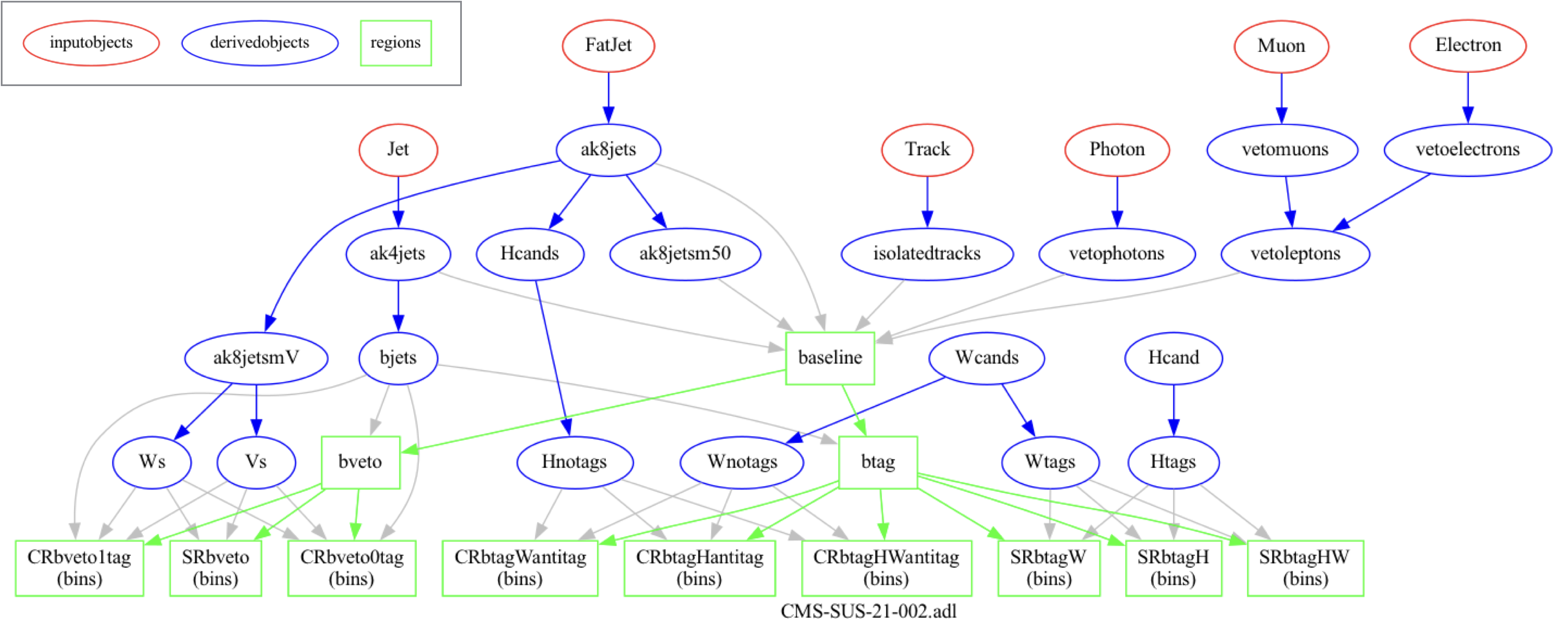
This analysis works with several different types of objects and multiple event selection regions, some of which are dependent on each other. Analyses we consider for reinterpretation are usually at least as complex as this one!
When we code such an analysis with a general purpose language, it becomes increasingly harder to visualize and keep track of the physics algorithm details. As the analysis physics content becomes more intricate, analysis code will become more complex, and harder to follow. It will be harder to trace, for example, which identification criteria define a certain object, which version of an object is used in which event selection region, etc.
The main reason behind this is that, when we write code using general purpose languages, we intertwine the physics algorithm with other technical details, e.g. accessing files, accessing variables, importing modules, etc. Despite the flexibility, all such technicalities obscure the code.
We present a modern method which allows to decouple physics algorithm from the technical code and write analyses with a simple, self-describing syntax. Analysis Description Language (ADL) is a HEP-specific analysis language developed with this purpose. Its main goal is to describe analyses in a more intuitive and physics-focused way. ADL is a transparant map from the input variables to the analysis selection.
Formal definition of ADL
More formally, ADL is a declarative domain specific language (DSL) that describes the physics content of a HEP analysis in a standard and unambiguous way.
- External DSL: Custom-designed syntax to express analysis-specific concepts. Reflects conceptual reasoning of particle physicists.
- Declarative: Tells what to do, but not how to do it.
- Human readable: Clear, self-describing syntax rules.
- Designed for everyone: experimentalists, phenomenologists, students, interested public…
Framework independence
ADL is designed to be framework-independent. Any framework recognizing ADL can perform tasks with it. Physics information becomes independent from software and framework details. This allows:
- Multi-purpose use of analysis description: Can be automatically translated or incorporated into the GPL / framework most suitable for a given purpose, e.g. exp, analysis, (re)interpretation, analysis queries, …
- Efficient communication between groups: experimentalists, phenomenologists, referees, students, public, …
- Accessible preservation of analysis physics logic.
Context and syntax
ADL mainly focuses on describing event processing. This includes object selections, event variable definitions and event selections. It can also described histogramming, and partially systematic uncertainties.
ADL consists of blocks separating object, variable and event selection definitions for a clear separation of analysis components. Blocks have a keyword-expression structure. Keywords specify analysis concepts and operations. Syntax includes mathematical and logical operations, comparison and optimization operators, reducers, 4-vector algebra and HEP-specific functions (dphi, dR, etc.).
ADL is designed with the goal to be self-describing, so especially for simple cases, one does not need to read syntax rules to understand an ADL description. However if you are interested, the set of syntax rules can be found here.
A physics analysis database
ADL is a standard, which allows all analyses to be described in the same way. Having access to many analyses written in the same way can help us understand them easier, learn their physics logic easily, and use them in our own studies.
All these design principles make ADL an excellent medium for reinterpretation studies.
What is CutLang?
Once an analysis is written it needs to be run on events. This is achieved by CutLang , the runtime interpreter that reads and understands the ADL syntax and runs it on events. A runtime interpreter does not require to be compiled. The user only modifies the ADL description, and runs CutLang. CutLang is also a framework which automatically handles many tedious tasks as reading input events, writing output histograms, etc. CutLang can be run on various environments such as linux, mac, conda, docker, jupyter, etc.
In case you are interested to learn more about CutLang, please see the CutLang github and references in the cern.ch/adl) portal.
Key Points
ADL is a declarative domain specific language (DSL) that describes the physics content of a HEP analysis in a standard and unambiguous way.
ADL’s purpose is to decouple the physics logic of analyses from technical operations, and make the physics logic more accessible.
CutLang is a runtime interpreter that reads and understands the ADL syntax and runs it on events.
Installing CutLang
Overview
Teaching: 0 min
Exercises: 40 minQuestions
How do I access information about CutLang in general?
How do I install CutLang via Docker?
How do I test my installation?
Can I already run some ADL examples with CutLang?
Objectives
Setup CutLang via Docker.
Understand the most basic concepts about running CutLang.
Perform a test run with CutLang on an open data POET ntuple and check the output.
Run a tutorial based on several ADL files in order to familiarize with the ADL syntax.
Prerequsite: Familiarity with Docker
Please make sure that you have followed the Docker pre-exercises and are familiar with Docker containers.
Please make sure that you prepare the CutLang setup before the next exercise.
Installing CutLang: introduction
CutLang is the runtime interpreter we will use for processing ADL files on events.
CutLang is compatible multiple platforms. It can be installed directly on Linux and MacOS, on all platforms via Docker or Conda, or can be accessed via a Jupyter/Binder interface.
The generic and most up-to-date instructions for setting up CutLang can be found in the CutLang github readme
In this exercise, we will use run CutLang via a docker container as described in the next section.
CutLang setup via Docker
Setup and execute
We have prepared a CutLang docker container which functions similarly to other Docker containers that work with CMS Open Data. The setup contains:
- CutLang
- ROOT
- xrootd access to open data ntuples
- VNC
- Jupyter
If you have an apple M1/M2 chip follow these instructions first:
Do the setup:
- In finder, go to
/Applications/Utilities- right click on Terminal and get its info
- in the info panel, tick “Open using Rosetta”
- (re)start the terminal application. Check your setup:
- Open a terminal and type
uname -a- Make sure you see
×86_64Once you have successfully done this setup, you should be able to work with the following instructions.
1. As a first step, make sure that you have Docker desktop installed.
You can find detailed instructions on how to install Docker and on simple Docker concepts and commands in this tutorial.
2. Next, download the CutLang image and run container in current directory from the downloaded image
For linux/MacOS:
docker run -p 8888:8888 -p 5901:5901 -p 6080:6080 -d -v $PWD/:/src --name CutLang-root-vnc cutlang/cutlang-root-vnc:latest
If you would like to re-run by mounting another directory, you should stop the container using
docker stop CutLang-root-vnc && docker container rm CutLang-root-vncand rerun with a different path as
docker run -p 8888:8888 -p 5901:5901 -p 6080:6080 -d -v /path/you/want/:/src .... For example:docker run -p 8888:8888 -p 5901:5901 -p 6080:6080 -d -v ~/example_work_dir/:/src --name CutLang-root-vnc cutlang/cutlang-root-vnc:latest
For Windows:
docker run -p 8888:8888 -p 5901:5901 -p 6080:6080 -d -v %cd%/:/src --name CutLang-root-vnc cutlang/cutlang-root-vnc:latest
If you would like to re-run by mounting another directory, you should stop the container using
docker stop CutLang-root-vnc && docker container rm CutLang-root-vncand rerun with a different path as
docker run -p 8888:8888 -p 5901:5901 -p 6080:6080 -d -v /path/you/want/:/src .... For example:docker run -p 8888:8888 -p 5901:5901 -p 6080:6080 -d -v ~/example_work_dir/:/src --name CutLang-root-vnc cutlang/cutlang-root-vnc:latest
3. Execute the container using
docker exec -it CutLang-root-vnc bash
If you have installed the container successfully, you will see
For examples see /CutLang/runs/
and for LHC analysis implementations, see
https://github.com/ADL4HEP/ADLLHCanalyses
Now, the container is ready to run CutLang.
You can leave the container by typing
exit
Update (if relevant)
In case an update is necessary, you can perform the update as follows:
docker pull cutlang/cutlang-root-vnc:latest
docker stop CutLang-root-vnc && docker container rm CutLang-root-vnc
docker run -p 8888:8888 -p 5901:5901 -p 6080:6080 -d -v $PWD/:/src --name CutLang-root-vnc cutlang/cutlang-root-vnc
Then execute, as usual:
docker exec -it CutLang-root-vnc bash
Remove
The CutLang docker container and image can be removed using
docker stop CutLang-root-vnc
docker ps -a | grep "CutLang-root-vnc" | awk '{print $1}' | xargs docker rm
docker images -a | grep "cutlang-root-vnc" | awk '{print $3}' | xargs docker rmi
Starting VNC and Jupyter
Starting VNC
VNC works similarly as in the other containers for CMS Open Data (described in this tutorial). Once in the CutLang container, type
start_vnc
You will see
VNC connection points:
	VNC viewer address: 127.0.0.1::5901
	HTTP access: http://127.0.0.1:6080/vnc.html
Copy the http address to your web browser and click connect. Note that the vnc password is different for this exercise.
VNC password
cutlang-adl
Before leaving the container, please stop vnc using the command
stop_vnc
Starting Jupyter
We will do some plotting using pyROOT. The plotting scripts can also be directly edited and run at commandline, but we will use Jupyter for this exercise. Once in the container, type the command
CLA_Jupyter lab
If all went well, you will see an output whose last few lines look as follows:
    To access the server, open this file in a browser:
        file:///home/cmsusr/.local/share/jupyter/runtime/jpserver-158-open.html
    Or copy and paste one of these URLs:
        http://da22da048c0d:8888/lab?token=c56366692a641a939320264a79dcb23a7a962e202896f5c0
     or http://127.0.0.1:8888/lab?token=c56366692a641a939320264a79dcb23a7a962e202896f5c0
Now open a browser window and copy the http address at the last line, e.g. starting with http://127..... into the browser. You will see that a jupyter notebook opens.
In order to exit the Jupyter setup and go back to the container commandline, press ctrl-c, and when prompted hutdown this Jupyter server (y/[n])?, type y.
Run CutLang
In the CutLang Docker container, type
CLA
If all went well, you will see the following output:
/CutLang/runs/CLA.sh
/CutLang/runs
/CutLang
ERROR: not enough arguments
/CutLang/runs/CLA.sh ROOTfile_name ROOTfile_type [-h]
    -i|--inifile
    -e|--events
    -s|--start
    -h|--help
    -d|--deps
    -v|--verbose
    -j|--parallel
ROOT file type can be:
 "LHCO"
 "FCC"
 "POET"
 "DELPHES2"
 "LVL0"
 "DELPHES"
 "ATLASVLL"
 "ATLMIN"
 "ATLTRT"
 "ATLASOD"
 "ATLASODR2"
 "CMSOD"
 "CMSODR2"
 "CMSNANO"
 "VLLBG3"
 "VLLG"
 "VLLF"
 "VLLSIGNAL"
This output explains us how to run CutLang. We need to provide the following inputs:
- input ROOT file containing events.
ROOTfile_namespecifies the address of this file.- We also need to specify the type of this ROOT file, i.e. the format of the events, via
ROOTfile_type. You can see above that CutLang automatically recognizes ROOT files with many different formats. For this exercise, our input are of thePOETtype.
- We also need to specify the type of this ROOT file, i.e. the format of the events, via
- ADL file with the analysis description. The ADL file is input via the
-iflag.
There are also optional flags to specify run properties. Here are two practical examples:
-e: Number of events to run. For example,-e 10000means we run only over 10000 events.-d: Enables a more efficient handling of dependent regions. Reduces runtime by 20-30 percent.
Now let’s try running CutLang!
For this test run, we will use a simple ADL file called /CutLang/runs/tutorials/ex00_helloworld.adl. First, open this ADL file using nano or vi to see how it has described a very simple object and event selection. It should be quite self-descriptive!
For input events, we will use a POET open data simulation sample: root://eospublic.cern.ch//eos/opendata/cms/derived-data/POET/23-Jul-22/RunIIFall15MiniAODv2_TprimeTprime_M-800_TuneCUETP8M1_13TeV-madgraph-pythia8_flat.root
Now, run CutLang with the folloing command:
CLA root://eospublic.cern.ch//eos/opendata/cms/derived-data/POET/23-Jul-22/RunIIFall15MiniAODv2_TprimeTprime_M-800_TuneCUETP8M1_13TeV-madgraph-pythia8_flat.root POET -i /CutLang/runs/tutorials/ex00_helloworld.adl -e 10000
WARNING: Please ignore the file does not exist message saying root://eospublic.cern.ch//eos/opendata/cms/derived-data/POET/23-Jul-22/RunIIFall15MiniAODv2_TprimeTprime_M-800_TuneCUETP8M1_13TeV-madgraph-pythia8_flat.root does not exist.
If CutLang runs successfully, you will see an output that ends as follows:
number of entries 10000
starting entry 0
last entry 10000
Processing event 0
Processing event 5000
Efficiencies for analysis : BP_1
						preselection	Based on 10000 events:
                                                               ALL :      1 +-         0 evt:    10000
                                                size(goodjets) > 3 :  0.971 +-   0.00168 evt:     9710
                                             pt(goodjets[0]) > 300 : 0.7748 +-   0.00424 evt:     7523
                                             pt(goodjets[1]) > 200 : 0.8551 +-   0.00406 evt:     6433
                                             pt(goodjets[2]) > 100 : 0.9431 +-   0.00289 evt:     6067
                                                    [Histo] hnjets :      1 +-         0 evt:     6067
                                                   [Histo] hjet1pt :      1 +-         0 evt:     6067
                                                   [Histo] hjet2pt :      1 +-         0 evt:     6067
					 --> Overall efficiency	 =   60.7 % +-  0.488 %
Bins for analysis : BP_1
saving...	saved.
finished.
CutLang finished successfully, now adding histograms
hadd Target file: /src/histoOut-CMSOD-hello-world.root
hadd compression setting for all output: 1
hadd Source file 1: /src/histoOut-BP_1.root
hadd Target path: /src/histoOut-ex00-helloworld.root:/
hadd Target path: /src/histoOut-ex00-helloworld.root:/preselection
hadd finished successfully, now removing auxiliary files
end CLA single
OPTIONAL: Copying events file to local
If you are connecting from outside CERN, it may take a while, e.g. several minutes for CutLang to access the file and start processing events. To make things faster, > you can alternatively copy the events file to your local directory and run on this local file.
You can copy the file using the
xrtdcpcommandxrdcp root://eospublic.cern.ch//eos/opendata/cms/derived-data/POET/23-Jul-22/RunIIFall15MiniAODv2_TprimeTprime_M-800_TuneCUETP8M1_13TeV-madgraph-pythia8_flat.root .then run CutLang as
CLA RunIIFall15MiniAODv2_TprimeTprime_M-800_TuneCUETP8M1_13TeV-madgraph-pythia8_flat.root POET -i /CutLang/runs/tutorials/ex00_helloworld.adl -e 10000
Look at this output and try to understand what happened during the event selection.
You should also get an output ROOT file histoOut-ex00-helloworld.root that contains the histograms you made and some further information.
Start VNC, if you have not already done so. Then open the root file and run a TBrowser:
root -l histoOut-ex00-helloworld.root
new TBrowser
Go to your web browser, where you should see the TBrowser open. Click on the histoOut-ex00-helloworld.root file, then on the preselection directory.
You will see the histograms you made in the preselection directory. Click on each histogram and look at the content.
You will also see another (automatically created) histogram called cutflow, which shows the event selection steps and events remaining after each step.
When you are done, you can quit the ROOT interpreter by .q.
Congratulations! Now you are ready to run ADL analyses via CutLang!
Run tutorials to familiarize with the ADL/CutLang syntax
ADL syntax is self-descriptive. Main syntax rules can be learned easily by studying and running a few tutorial examples.
These examples can be seen by ls /CutLang/runs/tutorials/*.adl
Let’s first download some simple event samples to run on the examples:
wget https://www.dropbox.com/s/ggi78bi4b6fv3r7/ttjets_NANOAOD.root
wget http://opendata.atlas.cern/release/samples/MC/mc_105986.ZZ.root
wget https://www.dropbox.com/s/zza28peyjy8qgg6/T2tt_700_50.root
The samples contain ttjets events in CMSNANO format, ZZto4lepton events in ATLASOD format and SUSY events in DELPHES format, respectively,
Please first look into each file and understand the algorithm and syntax. Then run the ADL files with the commands given below. If there are histograms made, check out the resulting ROOT file and inspect the histograms.
CLA ttjets_NANOAOD.root CMSNANO -i /CutLang/runs/tutorials/ex01_selection.adl
CLA ttjets_NANOAOD.root CMSNANO -i /CutLang/runs/tutorials/ex02_histograms.adl
CLA mc_105986.ZZ.root ATLASOD -i /CutLang/runs/tutorials/ex03_objreco.adl
CLA ttjets_NANOAOD.root CMSNANO -i /CutLang/runs/tutorials/ex04_syntaxes.adl
CLA T2tt_700_50.root DELPHES -i /CutLang/runs/tutorials/ex05_functions.adl
CLA T2tt_700_50.root DELPHES -i /CutLang/runs/tutorials/ex06_bins.adl
CLA ttjets_NANOAOD.root CMSNANO -i /CutLang/runs/tutorials/ex07_chi2optimize.adl
CLA ttjets_NANOAOD.root CMSNANO -i /CutLang/runs/tutorials/ex08_objloopsreducers.adl
CLA ttjets_NANOAOD.root CMSNANO -i /CutLang/runs/tutorials/ex09_sort.adl
CLA ttjets_NANOAOD.root CMSNANO -i /CutLang/runs/tutorials/ex10_tableweight.adl
CLA ttjets_NANOAOD.root CMSNANO -i /CutLang/runs/tutorials/ex11_printsave.adl
CLA T2tt_700_50.root DELPHES -i /CutLang/runs/tutorials/ex12_counts.adl
More ADL files for various full LHC analyses (focusing on signal region selections) can be found in this git repository.
Key Points
For up-to-date details for installing CutLang, the official documentation is the best bet.
Make sure you were able to setup CutLang via Docker and run its hello-world example.
Running CLA is the only thing that a user must know in order to work with CutLang.
The example ADL files in the
/CutLang/runs/tutorials/directory is the best way to immediately familiarize with the ADL syntax.
Open data reinterpretation with ADL/CutLang: ttbar to vector-like T quark
Overview
Teaching: 0 min
Exercises: 50 minQuestions
How can we do exact reinterpretation with open data and ADL/CutLang?
How can we do optimized reinterpretation with open data and ADL/CutLang?
How can we add analysis definitions to the ADL file?
How can we optimize an analysis, find discriminating variables?
What information we help us assess the adequacy of the analysis?
Objectives
Perform exact interpretation of a ttbar cross section analysis in a vector-like T quark signal using open data and ADL/CutLang.
Optimize the ttbar analysis to enhance sensitivity to the vector-like T quark signal using open data and ADL/CutLang.
Learn how to define new objects, new variables, new event selection cuts and new histograms in ADL.
Learn how to plot variable distributions and cutflows for different processes, weighted to the expected number of events at the LHC.
Prerequsite: CutLang-root-vnc Docker container and basic familiarity with running CutLang
The exercises here will be run in the CutLang docker container. Make sure you have followed Episode 3: Installing CutLang, have a working
CutLang-vnc-rootcontainer setup, and are able to run CutLang.
A familiar analysis for a new signal
In this exercise, we are going to take the top-antitop quark pair production analysis example you studied in the simplified analysis example session and use it to demonstrate a simple optimized reinterpretation case. We will modify the analysis selection, so that the analysis becomes sensitive to a new physics scenario, namely, vector-like quarks.
Let’s remember the top-antitop quark process, which was the original signal in the ttbar analysis:
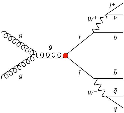 .
.
Now let’s see our new signal for reinterpretation, the vector-like top quark T, in its pair production mode, and with its decays:
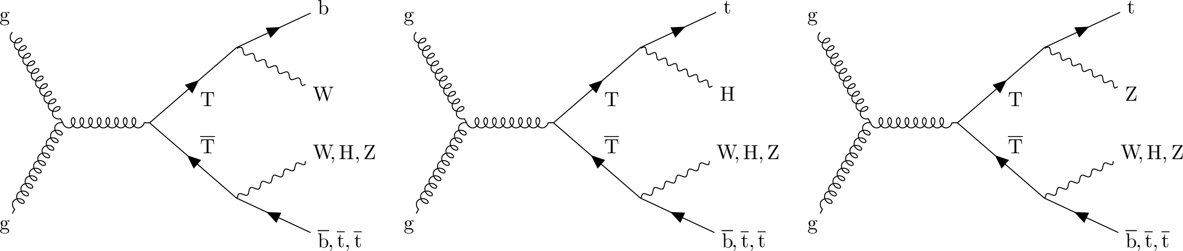 .
.
The vector-like T quark has similar properties with the SM top quark. For example, it can be pair produced, and decay to bW. But T can be much heavier. This opens different decays channels through Z and Higgs boson, as seen in the figure above. The heavier T gets, the more Lorentz boost its decay products receive. Our signal is a mixture of all the above decay channels. We will work with a signal benchmark with T mass = 800 GeV. We will also check results for two other benchmarks with T mass = 700 and 1200 GeV.
Exact reinterpretation
What happens if we reinterpreted the top-antitop analysis in terms of the vector-like T model? Is the analysis sensitive to the vector-like T signal? In order to find out, we must run the analysis on at least the signal events. It turns out, our signal events are available in open data, and even in POET format:
| T mass (GeV) | cross section (pb) | OD record | POET ntuple |
|---|---|---|---|
| 700 | 0.455 | 20232 | RunIIFall15MiniAODv2_TprimeTprime_M-700_TuneCUETP8M1_13TeV-madgraph-pythia8_flat.root |
| 800 | 0.196 | 20233 | RunIIFall15MiniAODv2_TprimeTprime_M-800_TuneCUETP8M1_13TeV-madgraph-pythia8_flat.root |
| 1200 | 0.0118 | 20225 | RunIIFall15MiniAODv2_TprimeTprime_M-1200_TuneCUETP8M1_13TeV-madgraph-pythia8_flat.root |
The POET ntuples have the prefix address: root://eospublic.cern.ch//eos/opendata/cms/derived-data/POET/23-Jul-22/ (add the root file name to the end).
Next comes the implementation of the analysis. We already have a version in ADL. Let’s download it to the docker container:
wget https://raw.githubusercontent.com/ADL4HEP/ADLAnalysisDrafts/main/CMSODWS23-ttbartovlq/ttbartovlq_step1.adl
Open the ADL file and see
- how the object definitions are written
- how the top candidate is reconstructed
- how the event selections are done for different regions and how the different regions are related
- how the histograms are defined for fixed binwidth and variable binwidth cases.
Discussion
What do you think about describing the analysis in this manner? Is it useful to see all the physics algorithm in one place?
Now let’s run the ADL file using CutLang over the Tmass = 800 GeV signal for 30000 events:
CLA root://eospublic.cern.ch//eos/opendata/cms/derived-data/POET/23-Jul-22/RunIIFall15MiniAODv2_TprimeTprime_M-800_TuneCUETP8M1_13TeV-madgraph-pythia8_flat.root POET -i ttbartovlq_step1.adl -e 30000
mv histoOut-ttbartovlq_step1.root histoOut-ttbartovlq_TT800.root
Look at the text output and the cutflow shown there. Which cuts reduce the events most?
Now let’s compare the top candidate mass from the signal with that of the ttbar process, which, in this case becomes our dominant background.
Event yields for various processes are usually provided with the analysis publication or in HepData, but in this case, we will get them ourselves. We can run the above ADL file on some ttbar events:
CLA root://eospublic.cern.ch//eos/opendata/cms/derived-data/POET/23-Jul-22/RunIIFall15MiniAODv2_TT_TuneCUETP8M1_13TeV-powheg-pythia8_flat.root POET -i ttbartovlq_step1.adl -e 500000
mv histoOut-ttbartovlq_step1.root histoOut-ttbartovlq_SMttbar.root
If accessing
ttbarevents is too slow for your setup, you can alternatively download thehistoOutfile that we prepared:wget --output-document=histoOut-ttbartovlq_SMttbar.root "https://www.dropbox.com/scl/fi/aptqbtwniuyj7les71al9/histoOut-ttbartovlq_SMttbar.root?rlkey=db5osn3i917g5zd4xc1u3meek&dl=0"
Next, let’s go to Jupyter and open a notebook to read the output ROOT files and draw histograms.
Assuming you are still in the default src/ directory of the docker container, go to the ../CutLang/binder directory and start Jupyter:
cd ../CutLang/binder/
CLA_Jupyter lab
(remember that you need to copy the url address at the bottom to your browser).
Tip for Jupyter
To make it easy to switch between Jupyter and the container prompt, you can work with two separate containers. You can do this by executing the container again in a different terminal shell by
docker exec -it CutLang-root-vnc bash.
Select the notebook ROOTweightedcomparison.ipynb. This notebook retrieves the set of histograms you select and plots them after applying weights that normalize them to cross section times luminosity. This means, the events in the histogram correspond to the event one would expect at the LHC.
Overview the code and execute the cells. You will see histograms appearing.
Discussion
Take a look at the top candidate mass distributions:
- Can this variable discriminate the signal from background?
- How does the signal / background ratio look? Do you think this selection is sensitive to our signal? Now take a look at the
cutflowhistograms. These are generated automatically by CutLang.- Is there any difference in event reduction rate between the signal and background?
Optimized reinterpretation
Finding and adding discriminating variables
We see that the ttbar analysis is not the best way to look for vector-like T quarks. Now let’s try to improve the selection to increase analysis sensitivity. To devise an improved selection, we should guess some variables with discriminating power and plot them for signal and background.
Discussion
What could be some signal discriminating variables? How could we determine them?
Main difference is that the signal events have a larger object multiplicity and decay products with bigger boost. This consequentally leads to larger transverse activity, both visible and invisible.
Challenge: Histogramming candidiate discriminating variables
Here are some ideas for discriminating variables. Please add histograms for these to the ADL file, under the
fourjettwobregion:
- Top quarks coming from T decays may have a large Lorentz boost, top candidate pT could be a discriminant.
- histogram name:
hpttop; fixed bins:20, 50, 1550- histogram name:
h2pttop: variable bins:50 100 150 200 300 400 500 600 700 800 1000 1500 2000- Signal should have higher jet multiplicity. Add number of jets.
- histogram name:
hnjets; fixed bins:20, 0, 20- pTs of the first 3 jets can be relatively higher. Add these three as separate histograms:
- histogram names:
hj1pT,hj2pT,hj3pT; fixed bins:20, 50, 1050- Signal can have larger MET. IMPORTANT: The variable to use for MET in ADL is simply
MET.
- histogram name:
hmet; variable bins:50 75 100 150 200 300 500 700 1000 1300- Signal can have larger visible transverse activity. A variable typically used is
ST, which equals to the sum of MET, pT of the first lepton and scalar sum of the pTs of all jets in the event.
- Add
STto the ADL file. Add the following lines just before the event selection:define ST = MET + pT(leptons[0]) + fHT(jets)You can use the variable
STin the event selection.- Add the
SThistogram with name:hST; variable bins:500 600 700 800 1000 1125 1500 1700 2000 2500 3000 4500- Signal has decays to boosted W, Z and Higgs bosons. Boosted objects can be clustered into large radius jets. Signal can have a larger number of large radius jets.
- Define an
AK8jetsobject in the ADL fille by adding the following object block to the object definitions section:object AK8jets take FJet select pT(FJet) > 200 select abs(Eta(FJet)) < 2.4 select m(FJet) > 60- Define an AK8jet multiplicity histogram with name:
hnak8; fixed bins:8, 0, 8Solution
 histo hpttop , "top cand. pT (GeV)", 20, 50, 1550, pT(topcands[0])
 histo h2pttop , "top cand. pT (GeV)", 50 100 150 200 300 400 500 600 700 800 1000 1500 2000, pT(to
pcands[0])
 histo hnjets , "number of jets", 20, 0, 20, size(jets)
 histo hj1pT , "jet 1 pT (GeV)", 20, 50, 1050, corrpT(jets[0])
 histo hj2pT , "jet 2 pT (GeV)", 20, 50, 1050, corrpT(jets[1])
 histo hj3pT , "jet 3 pT (GeV)", 20, 50, 1050, corrpT(jets[2])
 histo hmet , "MET (GeV)", 50 75 100 150 200 300 500 700 1000 1300, MET
 histo hST, "ST (GeV)", 500 600 700 800 1000 1125 1500 1700 2000 2500 3000 4500, ST
 histo hnak8, "number of AK8 jets", 8, 0, 8, size(AK8jets)
The complete ADL file after this step can be seen here.
Rerun the ADL file with CutLang on the signal, and if possible, ttbar background events as you had done above.
For ttbar events, if running is slow, you can continue using the
histoOut-ttbartovlq_ttjets.rootfile. It already contains all the histograms for this exercise, so it can be used to view the resulting histograms.
Go back to the Jupyter notebook. In the histoinfos list in the 4th cell, uncomment the names of the histograms you created. Rerun the notebook to obtain signal-background comparison histograms.
Discussion
- Which variables seem to have best discriminating power?
- What kind of cuts can we impose?
Defining and applying cuts
Time to add some cuts and see if the signal becomes more visible.
Challenge: Apply cuts
Let’s make a new
regionnamedoptforvlqreintthat inherits from thefourjettwobregion, and add the following cuts
- at least 1 AK8jet
- after this cut, add the following histograms:
histo hak8j1pT , "AK8 jet 1 pT (GeV)", 20, 200, 1200, pT(AK8jets[0]) histo h2ak8j1pT , "AK8 jet 1 pT (GeV)", 200 300 400 500 600 700 1000 1500 2000, pT(AK8jets[0]) histo hak8j1m , "AK8 jet 1 mass (GeV)", 18, 50, 500, m(AK8jets[0]) histo h2ak8j1m , "AK8 jet 1 mass (GeV)", 60 100 150 200 300 400 500, m(AK8jets[0])- at least 6 jets (regular jets)
- pT of the highest pT jet (with index 0) greater than 300 GeV.
- pT of the second highest pT jet (with index 1) greater than 150 GeV.
- pT of the third highest pT jet (with index 2) greater than 100 GeV.
- ST greater than 1500 GeV
- missing transverse energy greater than 75 GeV.
- after this cut, add the following histograms:
histo h2mtop2 , "top cand. mass (GeV)", 50 100 150 200 300 500 700 1000 2000, m(topcands[0])
histo h2pttop2 , "top cand. pT (GeV)", 50 100 150 200 300 400 500 600 700 800 1000 1500 2000, pT(topcands[0])
histo hmet2 , "MET (GeV)", 50 75 100 150 200 300 500 700 1000 1300, MET
histo hST2, "ST (GeV)", 500 600 700 800 1000 1125 1500 1700 2000 2500 3000 4500, ST
histo h2ak8j1pT2 , "AK8 jet 1 pT (GeV)", 200 300 400 500 600 700 1000 1500 2000, pT(AK8jets[0])
histo h2ak8j1m2 , "AK8 jet 1 mass (GeV)", 60 100 150 200 250 300 400 500, m(AK8jets[0])
Solution
The complete ADL file after this step can be seen here.
Once again, run this ADL file and check the new histograms in Jupyter.
Discussion
- The histograms after the last cut show the candidate variables for presenting the analysis result. Which one would you pick?
- Check the
cutflowhistogram in theoptforvlqreintregion. Do our cuts do a decent job in reducing the background while keeping as much signal as possible?
What changed along the way?
A unique strength of ADL is that it allows to straightforwardly document many versions of an analysis as you like, and make easy comparisons between different versions and track changes. We can do this even with a simple diff <oldversion.adl> <newversion.adl> command.
Let’s compare ADL files from the (original ttbar analysis with the optimized ttbartovlq analysis to easily overview what has changed along the way:
wget https://raw.githubusercontent.com/ADL4HEP/ADLAnalysisDrafts/main/CMSODWS23-ttbartovlq/ttbartovlq_step1.adl -P compareadls/
wget https://raw.githubusercontent.com/ADL4HEP/ADLAnalysisDrafts/main/CMSODWS23-ttbartovlq/ttbartovlq_step3.adl -P compareadls/
then
diff compareadls/ttbartovlq_step1.adl compareadls/ttbartovlq_step3.adl
(we downloaded ADL the files in order to not overwrite yours - you can also compare your own versions if you like)
We are developing dedicated tools to provide more informative comparisons.
Results in full glory: signal, background and data
Now that we have established a selection, it is time to see the performance and distributions for the full set of collision data, background Monte Carlo and signal Monte Carlo events. It is also good to check the performance for multiple signal benchmarks (with masses 700, 800, 1200 in our case).
To save time, we already ran all these samples with the latest ADL file. Download the output files under the /src/ directory and unpack:
wget --output-document=ttbartovlq-histoOuts.tgz "https://www.dropbox.com/scl/fi/ifs463djzyah5rtud88nh/ttbartovlq-histoOuts.tgz?rlkey=wnn3xajzx41aih3uxwi9zlc4r&dl=0"
tar -xzvf ttbartovlq-histoOuts.tgz
The set of samples processed, their cross sections and unskimmed number of events are listed in the file ttbartovlq-results/samples.txt.
Go to Jupyter again, and this time open the notebook ``. This notebook is very similar to the previous one. But this time, we plot all processes together, once again, with the correct weights. Run the notebook and enjoy observing the final histograms.
The end – or is it?
Congratulations! You have finished the exercise. We hope you enjoyed this simple reinterprtation study with ADL/CutLang and found it useful. We also hope you are inspired with ideas to start your own reinterpretation, or even new analysis design studies.
A dedicated VLQ analysis
In truth, CMS already has a dedicated analysis for vector-like quarks, which explore the boosted nature of decay products. CMS-B2G-16-024: Search for pair production of vector-like T and B quarks in single-lepton final states using boosted jet substructure in proton-proton collisions at sqrt(s) = 13 TeV arXiv link: (arXiv:1706.03408), publication reference: JHEP 11 (2017) 085 . Some cuts applied here were inspired by that analysis. In case you are curious, try our lesson on implementing that analysis from the 2022 workshop.
We are always happy to hear your suggestions and answer your questions!
Key Points
The ADL/CutLang allows practical and transparent implementation and optimization of an analysis for reinterpretation purposes using open data.
Optimized reinterpretation involves finding variables that discriminate signal from background; updating the event selection with cuts based on these discriminating variables; checking cutflows, variable distributions at various stages of the selection for high signal to background ratios; and finding a good final variable with the best signal to background ratio to express the analysis result.