Coffea Analysis
Overview
Teaching: 20 min
Exercises: 60 minQuestions
What is the general plan for the analysis?
What are the selection requirements?
How do I implement additional selection requirements?
What are Coffea Processors?
How do I run an analysis with Coffea?
Objectives
Understand the general strategy for the analysis
Learn how implement basic selection requirements
Learn how to build Coffea Processors and run an analysis
Prerequisites
For this episode please go to your
pythonDocker container and clone the repository for this exercise:git clone https://github.com/cms-opendata-workshop/workshop2022-lesson-ttbarljetsanalysis-payload.git cd workshop2022-lesson-ttbarljetsanalysis-payload
This episode is a recast of the analysis demo presented by Alexander Held at the IRIS-HEP AGC Workshop 2022. Our attempt is to make it more understandable by paying a bit more attention to the details. Note that this is work in progress and it will be refined in the future, perhaps using better consolidated ntuples (nanoAOD-like).
Datasets and pre-selection
As it was mentioned in the previous episode, we will be working towards a measurement of the top and anti-top quark production cross section \(\sigma_{t\bar{t}}\). The lepton+jets final state \(t\bar{t} \rightarrow (bW^{+})(\bar{b}W_{-}) \rightarrow bq\bar{q} bl^{-}\bar{\nu_{l}}\) is characterized by one lepton (here we look at electrons and muons only), significant missing transverse energy, and four jets, two of which are identified as b-jets.
For this analysis we will use the following datasets:
| type | dataset | variation | CODP name | xsec [pb] | size (TB) | Rec ID |
|---|---|---|---|---|---|---|
| colisions data | data | nominal | /SingleMuon/Run2015D-16Dec2015-v1/MINIAOD | 1.4 | 24119 | |
| /SingleElectron/Run2015D-08Jun2016-v1/MINIAOD | 2.6 | 24120 | ||||
| signal | ttbar | nominal | TT_TuneCUETP8M1_13TeV-powheg-pythia8 | 831.76 | 3.4 | 19980 |
| scaledown | TT_TuneCUETP8M1_13TeV-powheg-scaledown-pythia8 | 1.4 | 19983 | |||
| scaleup | TT_TuneCUETP8M1_13TeV-powheg-scaleup-pythia8 | 1.3 | 19985 | |||
| ME_var | TTJets_TuneCUETP8M1_13TeV-amcatnloFXFX-pythia8 | 1.3 | 19949 | |||
| PS_var | TT_TuneEE5C_13TeV-powheg-herwigpp | 0.8 | 19999 | |||
| backgrounds | single_top_t_chan | nominal | ST_t-channel_4f_leptonDecays_13TeV-amcatnlo-pythia8_TuneCUETP8M1 | 44.33 | 0.52 | 19397 |
| single_atop_t_chan | nominal | ST_t-channel_antitop_4f_leptonDecays_13TeV-powheg-pythia8_TuneCUETP8M1 | 26.38 | 0.042 | 19407 | |
| single_top_tW | nominal | ST_tW_top_5f_inclusiveDecays_13TeV-powheg-pythia8_TuneCUETP8M1 | 35.6 | 0.03 | 19419 | |
| ST_tW_antitop_5f_inclusiveDecays_13TeV-powheg-pythia8_TuneCUETP8M1 | 35.6 | 0.03 | 19412 | |||
| wjets | nominal | WJetsToLNu_TuneCUETP8M1_13TeV-amcatnloFXFX-pythia8 | 61526.7 | 3.8 | 20548 |
The nominal variation samples are the regular samples used in the analysis while samples corresonding to other variations are used for estimating systematic uncertainties. This will be discussed in the last episode.
As you can see, several of these datasets are quite large (TB in size), therefore we need to skim them. Also, as you were able to see previously, running CMSSW EDAnalyzers over these data (with the POET code, for instance) could be quite computing intensive. One could also estimate the time it would take to run over all the datasets we need using a single computer. To be efficient, you will need a computer cluster, but we will leave that for the Cloud Computing lesson. Fortunately, we have prepared these skims already at CERN, using CERN/CMS computing infrastructure. The skimmed files we will be using were obtained in essentially the same POET way, except that we applied some trigger filtering and some pre-selection requirements.
We explicitly required:
- That the events fired at least one of these triggers:
HLT_Ele22_eta2p1_WPLoose_Gsf,HLT_IsoMu20_v,HLT_IsoTkMu20_v. We assume these triggers were unprescaled, but you know now, one should really check (or ask!) - That the event contains either at least one tight electron with \(p_{T} > 26\) and \(\lvert\eta\rvert<2.1\) or at least one tight muon with \(p_{T} > 26\) and \(\lvert\eta\rvert<2.1\).
A json file called ntuples.json was created in order to keep track of these files and their metadata. You can find this file in your copy of the workshop2022-lesson-ttbarljetsanalysis-payload repository.
Building the basic analysis selection
Here we will attempt to build the histogram of a physical observable by implementing the physics object selection requirements that were used by the CMS analysts, who performed this analysis back in 2015. For understanding the basics of the analysis implementation, we will first attempt the analysis over just one collissions dataset (just one small file). Then, we will encapsulate our analysis in a Coffea processor and run it for all datasets: collisions (wich we will call just data), signal and background.
Here is a summary of the selection requirements used in the original CMS analysis:
Muon Selection
Exactly one muon
- \(p_T\) > 30 GeV, \(\lvert\eta\rvert<2.1\), tight ID
- relIso < 0.15 (corrected for pile-up contamination)
- SIP3D < 4
Electron Selection
Exactly one electron
- \(p_T\) > 30 GeV, \(\lvert\eta\rvert<2.1\), tight ID
- SIP3D < 4
Jet Selection
Require at least one jet
- Loose jet ID
- \(p_T\) > 30 GeV, \(\lvert\eta\rvert<2.4\), Fall15_25nsV2
- Jets identified as b-jets if CSV discriminator value > 0.8 (medium working point)
If for some reason you need to start over, take into account that the file
coffeaAnalysis_basics.py, in your copy of the exercise repository, contains all the relevant commands needed to complete the basic analysis part that is shown in this section.
Also remember, if you want to do work in a jupyter notebook you can start one with jupyter-lab --ip=0.0.0.0 --no-browser in your container.
Let’start fresh, import the needed libraries and open an example file (we include some additional libraries that will be needed):
import uproot
import numpy as np
import awkward as ak
import hist
import matplotlib.pyplot as plt
import mplhep as hep
from coffea.nanoevents import NanoEventsFactory, BaseSchema
from agc_schema import AGCSchema
events = NanoEventsFactory.from_root('root://eospublic.cern.ch//eos/opendata/cms/derived-data/POET/23-Jul-22/RunIIFall15MiniAODv2_TT_TuneCUETP8M1_13TeV-powheg-pythia8_flat/00EFE6B3-01FE-4FBF-ADCB-2921D5903E44_flat.root', schemaclass=AGCSchema, treepath='events').events()
We will apply the selection criteria and then make a meaningful histogram. Let’s divide the selection requirements into Objects selection and Event selection.
Objects selection
First, start by applying a \(p_{T}\) cut for the objects of interest, namely electrons, muons and jets. To compare, first check the number of objects in each subarray of the original collection:
ak.num(events.electron, axis=1)
ak.num(events.muon, axis=-1)
ak.num(events.jet, axis=1)
Before we go on, let’s do a quick check on the fields available for each of our objects of interest:
events.electron.fields
events.muon.fields
events.jet.fields
Now, let’s apply the \(p_{T}\) and \(\eta\) mask together with the tightness requirement for the leptons:
selected_electrons = events.electron[(events.electron.pt > 30) & (abs(events.electron.eta)<2.1) & (events.electron.isTight == True)]
selected_muons = events.muon[(events.muon.pt > 30) & (abs(events.muon.eta)<2.1) & (events.muon.isTight == True)]
selected_jets = events.jet[(events.jet.corrpt > 30) & (abs(events.jet.eta)<2.4)]
See what we got:
ak.num(selected_electrons, axis=1)
ak.num(selected_muons, axis=1)
ak.num(selected_jets, axis=1)
Note that the number of events are still the same, for example:
ak.num(events.electron, axis=0)
ak.num(selected_electrons, axis=0)
Also, check one particular subarray to see if the applied requirements make sense:
events.muon.pt[4]
events.muon.eta[4]
events.muon.isTight[4]
selected_muons.pt[4]
selected_muons.eta[4]
selected_muons.isTight[4]
Challenge: Adding isolation and sip3d requirements for leptons
Please resist the urge to look at the solution. Only compare with the proposed solution after you make your own attempt.
Redo the lepton selection above (for
selected_electrons,selected_muons) to include:
- The relIsolation requirement for the muons (the one we built for dealing with pile-up)
- The requirement for the Significance on the Impact Parameter in 3D (SIP3D) for muons and electrons
Solution
selected_electrons = events.electron[(events.electron.pt > 30) & (abs(events.electron.eta)<2.1) & (events.electron.isTight == True) & (events.electron.sip3d < 4)]
selected_muons = events.muon[(events.muon.pt > 30) & (abs(events.muon.eta)<2.1) & (events.muon.isTight == True) & (events.muon.sip3d < 4) & (events.muon.pfreliso04DBCorr < 0.15)]
Events selection
At this point it would be good to start playing around with the different methods that awkward gives you. Remember tha when exploring interactively, you could always type ak. and hit the Tab key to see the different methods available:
>>> ak.
Display all 123 possibilities? (y or n)
ak.Array(                  ak.awkward                 ak.from_arrow(             ak.kernels(                ak.operations              ak.strings_astype(         ak.types
ak.ArrayBuilder(           ak.behavior                ak.from_awkward0(          ak.layout                  ak.packed(                 ak.sum(                    ak.unflatten(
ak.ByteBehavior(           ak.behaviors               ak.from_buffers(           ak.linear_fit(             ak.pad_none(               ak.to_arrow(               ak.unzip(
ak.ByteStringBehavior(     ak.broadcast_arrays(       ak.from_categorical(       ak.local_index(            ak.parameters(             ak.to_arrow_table(         ak.validity_error(
ak.CategoricalBehavior(    ak.cartesian(              ak.from_cupy(              ak.mask(                   ak.partition               ak.to_awkward0(            ak.values_astype(
ak.CharBehavior(           ak.categories(             ak.from_iter(              ak.materialized(           ak.partitioned(            ak.to_buffers(             ak.var(
ak.Record(                 ak.combinations(           ak.from_jax(               ak.max(                    ak.partitions(             ak.to_categorical(         ak.virtual(
ak.Sized()                 ak.concatenate(            ak.from_json(              ak.mean(                   ak.prod(                   ak.to_cupy(                ak.where(
ak.StringBehavior(         ak.copy(                   ak.from_numpy(             ak.min(                    ak.ptp(                    ak.to_jax(                 ak.with_cache(
ak.all(                    ak.corr(                   ak.from_parquet(           ak.mixin_class(            ak.ravel(                  ak.to_json(                ak.with_field(
ak.any(                    ak.count(                  ak.from_regular(           ak.mixin_class_method(     ak.regularize_numpyarray(  ak.to_kernels(             ak.with_name(
ak.argcartesian(           ak.count_nonzero(          ak.full_like(              ak.moment(                 ak.repartition(            ak.to_layout(              ak.with_parameter(
ak.argcombinations(        ak.covar(                  ak.highlevel               ak.nan_to_num(             ak.run_lengths(            ak.to_list(                ak.without_parameters(
ak.argmax(                 ak.fields(                 ak.is_categorical(         ak.nplike                  ak.singletons(             ak.to_numpy(               ak.zeros_like(
ak.argmin(                 ak.fill_none(              ak.is_none(                ak.num(                    ak.size(                   ak.to_pandas(              ak.zip(
ak.argsort(                ak.firsts(                 ak.is_valid(               ak.numba                   ak.softmax(                ak.to_parquet(
ak.atleast_1d(             ak.flatten(                ak.isclose(                ak.numexpr                 ak.sort(                   ak.to_regular(
ak.autograd                ak.forms                   ak.jax                     ak.ones_like(              ak.std(                    ak.type(
You could also get some help on what they do by typing, in your interactive prompt, something like:
help(ak.count)
to obtain:
Help on function count in module awkward.operations.reducers:

count(array, axis=None, keepdims=False, mask_identity=False)
    Args:
        array: Data in which to count elements.
        axis (None or int): If None, combine all values from the array into
            a single scalar result; if an int, group by that axis: `0` is the
            outermost, `1` is the first level of nested lists, etc., and
            negative `axis` counts from the innermost: `-1` is the innermost,
            `-2` is the next level up, etc.
        keepdims (bool): If False, this reducer decreases the number of
            dimensions by 1; if True, the reduced values are wrapped in a new
            length-1 dimension so that the result of this operation may be
            broadcasted with the original array.
        mask_identity (bool): If True, reducing over empty lists results in
            None (an option type); otherwise, reducing over empty lists
            results in the operation's identity.

    Counts elements of `array` (many types supported, including all
    Awkward Arrays and Records). The identity of counting is `0` and it is
    usually not masked.

    This function has no analog in NumPy because counting values in a
    rectilinear array would only result in elements of the NumPy array's
    [shape](https://docs.scipy.org/doc/numpy/reference/generated/numpy.ndarray.shape.html).

    However, for nested lists of variable dimension and missing values, the
    result of counting is non-trivial. For example, with this `array`,

        ak.Array([[ 0.1,  0.2      ],
                  [None, 10.2, None],
                  None,
                  [20.1, 20.2, 20.3],
                  [30.1, 30.2      ]])

    the result of counting over the innermost dimension is

        >>> ak.count(array, axis=-1)
        <Array [2, 1, None, 3, 2] type='5 * ?int64'>

    the outermost dimension is

        >>> ak.count(array, axis=0)
        <Array [3, 4, 1] type='3 * int64'>

    and all dimensions is

        >>> ak.count(array, axis=None)
        8
Let’s work on the single lepton requirement. Remember, the criteria indicates that we will only consider events with exactly one electron or exactly one muon. Let’see how we can do this:
event_filters = ((ak.count(selected_electrons.pt, axis=1) + ak.count(selected_muons.pt, axis=1)) == 1)
In order to keep the analyisis regions (we will see this later) from the original AGC demo, let’s require at least four jets in our event filter:
event_filters = event_filters & (ak.count(selected_jets.corrpt, axis=1) >= 4)
Challenge: Require at least one b-tagged jet
Please resist the urge to look at the solution. Only compare with the proposed solution after you make your own attempt.
To the
event_filtersabove, add the requirement to have at least one b-tagged jet with score above the proposed threshold (medium point; see above)Solution
# at least one b-tagged jet ("tag" means score above threshold)
B_TAG_THRESHOLD = 0.8
event_filters = event_filters & (ak.sum(selected_jets.btag >= B_TAG_THRESHOLD, axis=1) >= 1)
Let’s now apply the event filters:
selected_events = events[event_filters]
selected_electrons = selected_electrons[event_filters]
selected_muons = selected_muons[event_filters]
selected_jets = selected_jets[event_filters]
Signal region selection
In a typical analysis one can construct a control region (with no essentially no expected signal) and a signal region (with signal events). Let’s call our signal region 4j2b, because the final state of the process we are aiming to measure has at least 4, two of which should be from b quarks.
Let’s define a filter for this region and create such region:
region_filter = ak.sum(selected_jets.btag > B_TAG_THRESHOLD, axis=1) >= 2
selected_jets_region = selected_jets[region_filter]
Now, here is where the true power of columnar analysis and the wonderful python tools that are being developed become really evident. Let’s reconstruct the hadronic top as the bjj system with the largest \(p_{T}\). We will get ourselves an observable, which is the mass.
trijet = ak.combinations(selected_jets_region, 3, fields=["j1", "j2", "j3"])  # trijet candidates
trijet["p4"] = trijet.j1 + trijet.j2 + trijet.j3  # calculate four-momentum of tri-jet system
trijet["max_btag"] = np.maximum(trijet.j1.btag, np.maximum(trijet.j2.btag, trijet.j3.btag))
trijet = trijet[trijet.max_btag > B_TAG_THRESHOLD]  # require at least one-btag in trijet candidates
# pick trijet candidate with largest pT and calculate mass of system
trijet_mass = trijet["p4"][ak.argmax(trijet.p4.pt, axis=1, keepdims=True)].mass
observable = ak.flatten(trijet_mass)
Challenge: Can you figure out what is happening above?
Take some time to understand the logic of the above statements and explore the awkward methods used to get the ovbservable.
Histogramming and plotting
More information on this topic, including a very instructive video, can be found in one of the tutorials of the IRIS-HEP AGC Tools 2021 Workshop. We will not go into the details here, but just show you some examples.
We will use Hist from the hist package.
So, now we have a flat array for our observable. What else do we need for plotting? Well, a histogram is essentially a way to reduce our data. We can’t just plot every value of trijet mass, so we divide up our range of masses into n bins across some reasonable range. Thus, we need to define the mapping for our reduction; defining the number of bins and the range is sufficient for this. This is called a Regular axis in the hist.Hist package.
In our case, let’s plot 25 bins between values of 50 and 550. Because a histogram can contain an arbitrary amount of axes, we also need to give our axis a name (which becomes its reference in our code) and a label (which is the label on the axis that users see when the histogram is plotted).
Since we will be using several datasets (for signal, background and collisions data) we need a wasy of keep these contributions separate in our histograms. One can del with this using Categorical axes. A Categorical axis takes a name, a label, and a pre-defined list of categories. Let’s book a generic histogram with such capabilities:
histogram = hist.Hist.new.Reg(25, 50, 550, name="observable", label="observable [GeV]").StrCat(["4j1b", "4j2b"], name="region", label="Region").StrCat([], name="process", label="Process", growth=True).StrCat([], name="variation", label="Systematic variation", growth=True).Weight()
This histogram placeholder is of type that can accep a Weight to the data tha goes in. This is because for simulated MC samples (backgrounds)
, we will need to normalize the number of events to the total integrated luminosity.
By the way, if you look at the documentation,
help(hist.Hist.new)
you will find
|  Reg = Regular(self, bins: 'int', start: 'float', stop: 'float', *, name: 'str' = '', label: 'str' = '', metadata: 'Any' = None, flow: 'bool' = True, underflow: 'bool | None' = None, overflow: 'bool | None'
= None, growth: 'bool' = False, circular: 'bool' = False, transform: 'AxisTransform | None' = None, __dict__: 'dict[str, Any] | None' = None) -> 'ConstructProxy'
 |
 |  Regular(self, bins: 'int', start: 'float', stop: 'float', *, name: 'str' = '', label: 'str' = '', metadata: 'Any' = None, flow: 'bool' = True, underflow: 'bool | None' = None, overflow: 'bool | None' = None
, growth: 'bool' = False, circular: 'bool' = False, transform: 'AxisTransform | None' = None, __dict__: 'dict[str, Any] | None' = None) -> 'ConstructProxy'
It is useful at this point to do:
histogram.ndim
histogram.axes
in order to understand the structure a bit better. You can see that this hist object is multidimensional holder for histograms, which makes it very convenient and very powerful. You could fill out the outter most StrCategories with several processes and variations. You can slice and dice. Here a very quick example: let’s say that, once the histogram is filled (we haven’t done that yet), you want to get the histograms which have to with the signal region. Accessing them is very simple:
histogram[:,1,:,:]
Now, let’s fill in the histogram:
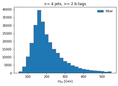
histogram.fill(observable=observable, region="4j2b", process="ttbar", variation="nominal", weight=1)
and then plot
histogram[:,"4j2b","ttbar","nominal"].plot(histtype="fill", linewidth=1, edgecolor="grey", label='ttbar')
plt.legend()
plt.title(">= 4 jets, >= 2 b-tags")
plt.xlabel("$m_{bjj}$ [Gev]");
plt.show()
Coffea Processors
We now see how simple it could be to construct an analysis using python tools. Naturally, we would like to scale it up to a far larger datasets in any practical scenario. So the first expansion we can do to our analysis is to consider running it over more datasets, which include all of our data, our background, and the signal. Additionally, we would like to show to how to *estimate a few sources of systematic uncertainty, and for that we will be using, in some cases, additional datasets. These systematics datasets are generaly variations of the nominal ones.
To expand our analysis, we will use coffea Processors. Processors are coffea’s way of encapsulating an analysis in a way that is deployment-neutral. Once you have a Coffea analysis, you can throw it into a processor and use any of a variety of executors (e.g. Dask, Parsl, Spark) to chunk it up and run it across distributed workers. This makes scale-out simple and dynamic for users. Unfortunately, we don’t have the time to do such a demostration, but we will run it locally, with our vanilla coffea executor.
Key Point
If you ever get to use executors that can parallelize across distributed workers (e.g., Dask, Parsl, Spark), note that we can do this in HEP. Events are independent of each other, so if we split our work up and ship it off to different workers, we aren’t violating the data’s integrity. Furthermore, since the output we seek is a histogram, our output is also independent of how the work is split up. As long as each worker maps its data to a histogram, the summation of those histograms will be identical to a single worker processing all of the data. In coffea, an object that behaves in this way is called an accumulator.
Defining our coffea Processor
The processor includes a lot of the physics analysis details:
- event filtering and the calculation of observables,
- event weighting,
- calculating systematic uncertainties at the event and object level,
- filling all the information into histograms that get aggregated and ultimately returned to us by coffea
In the coffeaAnalysis_ttbarljets.py in your copy of the repository you will find the definition of our Processor. It is built as a python class, which nicely encapsulates it and, as advertised, becomes independent of the executor.
Inspect it briefly, you will recognize the basic ingredients that we already explored. The only difference is that it has been modified so it allows for additional features like running over different processes and/or variations of them and filling in corresponding histograms.
Take a look at the Processor implementation
Open the Processor
#------------------------------------
class TtbarAnalysis(processor_base):
#------------------------------------
    #--------------------
    def __init__(self):
    #--------------------
        num_bins = 25
        bin_low = 50
        bin_high = 550
        name = "observable"
        label = "observable [GeV]"
        #https://hist.readthedocs.io/en/latest/user-guide/quickstart.html
        #StrCat = StrCategory
        #https://hist.readthedocs.io/en/latest/banner_slides.html?highlight=StrCategory#many-axis-types
        self.hist = (
            hist.Hist.new.Reg(num_bins, bin_low, bin_high, name=name, label=label)
            .StrCat(["4j1b", "4j2b"], name="region", label="Region")
            .StrCat([], name="process", label="Process", growth=True)
            .StrCat([], name="variation", label="Systematic variation", growth=True)
            .Weight()
        )
    #-------------------------
    def process(self, events):
    #-------------------------
        histogram = self.hist.copy()

        process = events.metadata["process"]  # "ttbar" etc.
        variation = events.metadata["variation"]  # "nominal", "scaledown", etc.

        #print(f'Currently doing variation {variation} for {process}')

        # normalization for MC
        x_sec = events.metadata["xsec"]
        nevts_total = events.metadata["nevts"]
        # This truelumi number was obtained with
# brilcalc lumi -c web -i Cert_13TeV_16Dec2015ReReco_Collisions15_25ns_JSON_v2.txt -u /pb --normtag normtag_PHYSICS_2015.json  --begin 256630 --end 260627 > lumi2015D.txt
        # lumi in units of /pb
        lumi = 2256.38
        if process != "data":
            xsec_weight = x_sec * lumi / nevts_total
        else:
            xsec_weight = 1

        #### systematics
        # example of a simple flat weight variation, using the coffea nanoevents systematics feature
        # https://github.com/CoffeaTeam/coffea/blob/20a7e749eea3b8de4880088d2f0e43f6ef9d7993/coffea/nanoevents/methods/base.py#L84
        # Help on method add_systematic in module coffea.nanoevents.methods.base:
        # add_systematic(name: str, kind: str, what: Union[str, List[str], Tuple[str]], varying_function: Callable)
        # method of coffea.nanoevents.methods.base.NanoEventsArray instance
        if process == "wjets":
            events.add_systematic("scale_var", "UpDownSystematic", "weight", flat_variation)

        # example on how to get jet energy scale / resolution systematics
        # need to adjust schema to instead use coffea add_systematic feature, especially for ServiceX
        # cannot attach pT variations to events.jet, so attach to events directly
        # and subsequently scale pT by these scale factors
        events["pt_nominal"] = 1.0
        #events["pt_scale_up"] = 1.03
        # we have already these corrections in our data for this workshop, so we might as well use them
        # to assign a variation per jet and not per event. However, to avoid messing too much with this code,
        # try a silly thing just for fun: take the average of jet variations per event (fill out the None values with a default 1.03)
        events['pt_scale_up'] = ak.fill_none(ak.mean(events.jet.corrptUp/events.jet.corrpt,axis=1),1.03)
        events["pt_res_up"] = jet_pt_resolution(events.jet.corrpt)

        pt_variations = ["pt_nominal", "pt_scale_up", "pt_res_up"] if variation == "nominal" else ["pt_nominal"]
        for pt_var in pt_variations:

            ### event selection
            # based on https://link.springer.com/article/10.1007/JHEP09(2017)051

            #object filters
            > > selected_electrons = events.electron[(events.electron.pt > 30) & (abs(events.electron.eta)<2.1) & (events.electron.isTight == True) & (events.electron.sip3d < 4)]
            > > selected_muons = events.muon[(events.muon.pt > 30) & (abs(events.muon.eta)<2.1) & (events.muon.isTight == True) & (events.muon.sip3d < 4) & (events.muon.pfreliso04DBCorr < 0.15)]
            jet_filter = (events.jet.corrpt * events[pt_var] > 30) & (abs(events.jet.eta)<2.4)
            selected_jets = events.jet[jet_filter]

            # single lepton requirement
            event_filters = ((ak.count(selected_electrons.pt, axis=1) + ak.count(selected_muons.pt, axis=1)) == 1)
            # at least four jets
            pt_var_modifier = events[pt_var] if "res" not in pt_var else events[pt_var][jet_filter]
            event_filters = event_filters & (ak.count(selected_jets.corrpt * pt_var_modifier, axis=1) >= 4)
            # at least one b-tagged jet ("tag" means score above threshold)
            B_TAG_THRESHOLD = 0.8
            event_filters = event_filters & (ak.sum(selected_jets.btag >= B_TAG_THRESHOLD, axis=1) >= 1)

            # apply event filters
            selected_events = events[event_filters]
            selected_electrons = selected_electrons[event_filters]
            selected_muons = selected_muons[event_filters]
            selected_jets = selected_jets[event_filters]

            for region in ["4j1b", "4j2b"]:
                # further filtering: 4j1b CR with single b-tag, 4j2b SR with two or more tags
                if region == "4j1b":
                    region_filter = ak.sum(selected_jets.btag >= B_TAG_THRESHOLD, axis=1) == 1
                    selected_jets_region = selected_jets[region_filter]
                    # use HT (scalar sum of jet pT) as observable
                    pt_var_modifier = events[event_filters][region_filter][pt_var] if "res" not in pt_var else events[pt_var][jet_filter][event_filters][region_filter]
                    observable = ak.sum(selected_jets_region.corrpt * pt_var_modifier, axis=-1)

                elif region == "4j2b":
                    region_filter = ak.sum(selected_jets.btag > B_TAG_THRESHOLD, axis=1) >= 2
                    selected_jets_region = selected_jets[region_filter]

                    # reconstruct hadronic top as bjj system with largest pT
                    # the jet energy scale / resolution effect is not propagated to this observable at the moment
                    trijet = ak.combinations(selected_jets_region, 3, fields=["j1", "j2", "j3"])  # trijet candidates
                    trijet["p4"] = trijet.j1 + trijet.j2 + trijet.j3  # calculate four-momentum of tri-jet system
                    trijet["max_btag"] = np.maximum(trijet.j1.btag, np.maximum(trijet.j2.btag, trijet.j3.btag))
                    trijet = trijet[trijet.max_btag > B_TAG_THRESHOLD]  # require at least one-btag in trijet candidates
                    # pick trijet candidate with largest pT and calculate mass of system
                    trijet_mass = trijet["p4"][ak.argmax(trijet.p4.pt, axis=1, keepdims=True)].mass
                    observable = ak.flatten(trijet_mass)

                ### histogram filling
                if pt_var == "pt_nominal":
                    # nominal pT, but including 2-point systematics
                    histogram.fill(
                            observable=observable, region=region, process=process, variation=variation, weight=xsec_weight
                        )


                    if variation == "nominal":
                        # also fill weight-based variations for all nominal samples
                        # this corresponds to the case for wjets included above as an example
                        for weight_name in events.systematics.fields:
                            for direction in ["up", "down"]:
                                # extract the weight variations and apply all event & region filters
                                weight_variation = events.systematics[weight_name][direction][f"weight_{weight_name}"][event_filters][region_filter]
                                # fill histograms
                                histogram.fill(
                                    observable=observable, region=region, process=process, variation=f"{weight_name}_{direction}", weight=xsec_weight*weight_variation
                                )

                        # calculate additional systematics: b-tagging variations
                        for i_var, weight_name in enumerate([f"btag_var_{i}" for i in range(4)]):
                            for i_dir, direction in enumerate(["up", "down"]):
                                # create systematic variations that depend on object properties (here: jet pT)
                                if len(observable):
                                    weight_variation = btag_weight_variation(i_var, selected_jets_region.corrpt)[:, i_dir]
                                else:
                                    weight_variation = 1 # no events selected
                                histogram.fill(
                                    observable=observable, region=region, process=process, variation=f"{weight_name}_{direction}", weight=xsec_weight*weight_variation
                                )

                elif variation == "nominal":
                    # pT variations for nominal samples
                    histogram.fill(
                            observable=observable, region=region, process=process, variation=pt_var, weight=xsec_weight
                        )
        output = {"nevents": {events.metadata["dataset"]: len(events)}, "hist": histogram}

        return output
    # https://coffeateam.github.io/coffea/api/coffea.processor.ProcessorABC.html?highlight=postprocess#coffea.processor.ProcessorABC.postprocess
    def postprocess(self, accumulator):
        return accumulator
Right below this Processor class, in the coffeaAnalysis_ttbarljets.py file, you will find a snippet which builds the input for the Processor (i.e., for the analysis):
# "Fileset" construction and metadata via utils.py file
# Here, we gather all the required information about the files we want to process: paths to the files and asociated metadata
# making use of the utils.py code in this repository
fileset = construct_fileset(N_FILES_MAX_PER_SAMPLE, use_xcache=False)
print(f"processes in fileset: {list(fileset.keys())}")
print(f"\nexample of information in fileset:\n { {\n  'files': [{fileset['ttbar__nominal']['files'][0]}, ...],")
print(f"  'metadata': {fileset['ttbar__nominal']['metadata']}\n } }")
t0 = time.time()
This is done with the help of the function construct_fileset, which is part of the utils.py file that you can also find in the repository. After you import the code in this file (like it is done in the heade of coffeaAnalysis_ttbarljets.py),
# Slimmed version of:
# https://github.com/iris-hep/analysis-grand-challenge/tree/main/analyses/cms-open-data-ttbar/utils
# These file contain code for bookkeeping and cosmetics, as well as some boilerplate
from utils import *
you get some utilities like styling routines and the fileset builder. Note that it is here where the cross sections for the different samples are stored. Also, the ntuples.json file (also find it in the repository) is read here to manage the fileset that will be fed to the Processor. We do some gymnastics also to adjust the normalization correctly. Finally there is a function to save the histograms in a ROOT file.
Next, in the coffeaAnalysis_ttbarljets.py file, you will see the call-out for the executor:
#Execute the data delivery pipeline
#we don't have an external executor, so we use local coffea (IterativeExecutor())
if PIPELINE == "coffea":
    executor = processor.IterativeExecutor()
    from coffea.nanoevents.schemas.schema import auto_schema
    schema = AGCSchema if PIPELINE == "coffea" else auto_schema
    run = processor.Runner(executor=executor, schema=schema, savemetrics=True, metadata_cache={})
    all_histograms, metrics = run(fileset, "events", processor_instance=TtbarAnalysis())
    all_histograms = all_histograms["hist"]
It is here where you decide where to run. Unfortunately, the datasets over which we are running are still quite large. So running on the whole dataset in a single computer is not very efficient. It will take a long time. Here is where coffea really performs, because you can ship it to different worker nodes using some different executors.
Finally note that there are some auxiliary functions at the beginning of the coffeaAnalysis_ttbarljets.py file and some histogramming routines at the end. We won’t worry about them for now.
Running an example of the analysis
If you have a good connection you may get to run over just a single file per dataset by setting the N_FILES_MAX_PER_SAMPLE = 1 at the beggining of the coffeaAnalysis_ttbarljets.py file. Otherwise, do not worry we will provide you with the final histograms.root output after we ran over the whole dataset (for reference, it takes about 4 hours in a regular laptop).
Let’s run the demonstrator:
python coffeaAnalysis_ttbarljets.py
While we wait, explore all these files
Feel free to take time to explore the files that complement the analysis infrastructure. Ask a a question!
Plotting
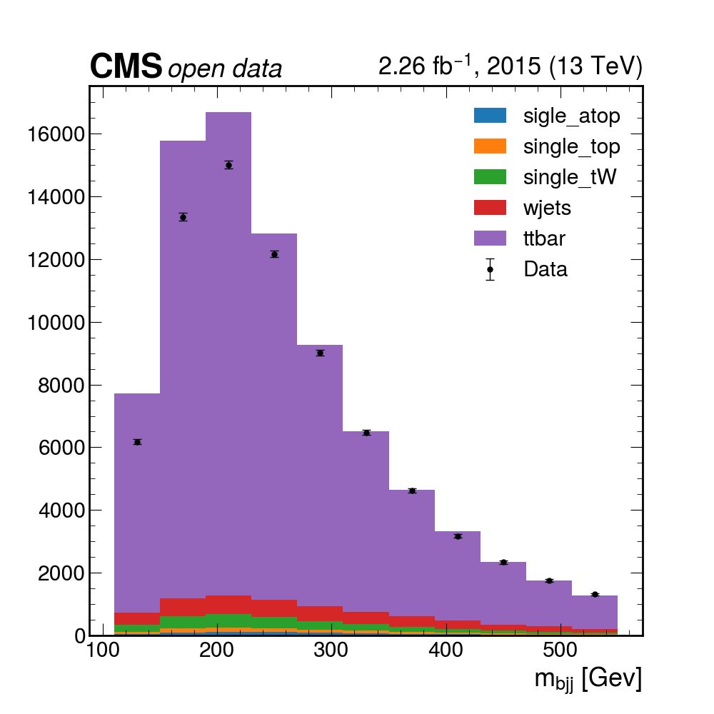
Plotting the final results
Here you can download a full
histograms.root. It was obtained after 4 hours of running on a single computer. Of course, if you have some available space, you could download the files (the size is not terribly large, maybe around 60GB or so), and run much faster. It contains all the histograms produced by the analysis Processor. We have prepared a plotting script for you to see the results:python plotme.py
Key Points
Basic selection requirements are implemented very easily using columnar analysis
Coffea processors encapsulate an analysis so it becomes deployment-neutral