General Physics Objects and POET

Overview

Teaching: 20 min
Exercises: 40 min

Questions

• What do we call physics objects in CMS?

• How are physics objects reconstructed?

• What is POET?

• How do I run POET?

Objectives

• Learn about the different physics objects in CMS and get briefed on their reconstruction

• Learn what the POET software is and how to run it

• Learn the structure of the POET configurator and how add new physics objects.

Overview

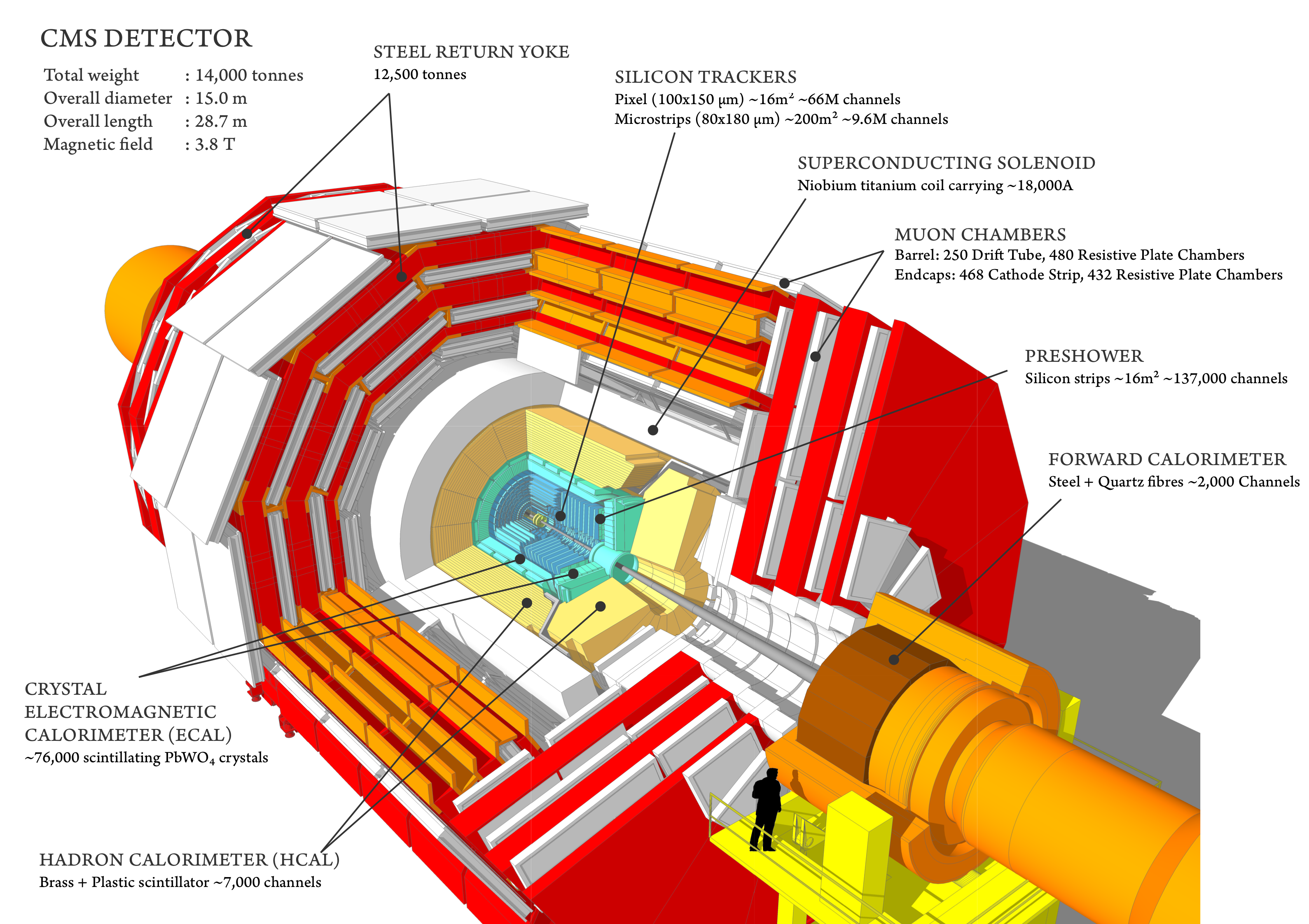
The CMS experment is a giant detector that acts like a camera that “photographs” particle collisions, allowing us to interpret their nature.

Certainly, we cannot directly observe all the particles created in the collisions because some of them decay very quickly or simply do not interact with our detector. However, we can infer their presence. If they decay to other stable particles and interact with the apparatus, they leave signals in the CMS subdetectors. These signals are used to reconstruct the decay products or infer their presence; we call these, physics objects.

Physics objects are built with the information collected by the sensors of the CMS detector. Take a look at the CMS experiment in the image below. This is a good recent video that you can watch later to get a quick feeling of how CMS looks now in Run 3.

Physics objects could be

•   muons
•   electrons
•   jets
•   photons
•   taus
•   missing transverse momentum

For the current releases of open data, we store them in ROOT files following the EDM data model in the so-called miniAOD format. One needs the CMSSW software to read and extract information (of the physics objects) from these files.

In the CERN Open Portal (CODP) site one can find a more detailed description of these physical objects and a list of them corresponding to 2010, 2011/2012 from Run 1, and 2015 (Run 2) releases of open data.

In this workshop we will focus on working with open data from the latest 2015 release from Run 2. However, you will get a taste of using Run 1 data as well, tomorrow.

Physics Objects reconstruction

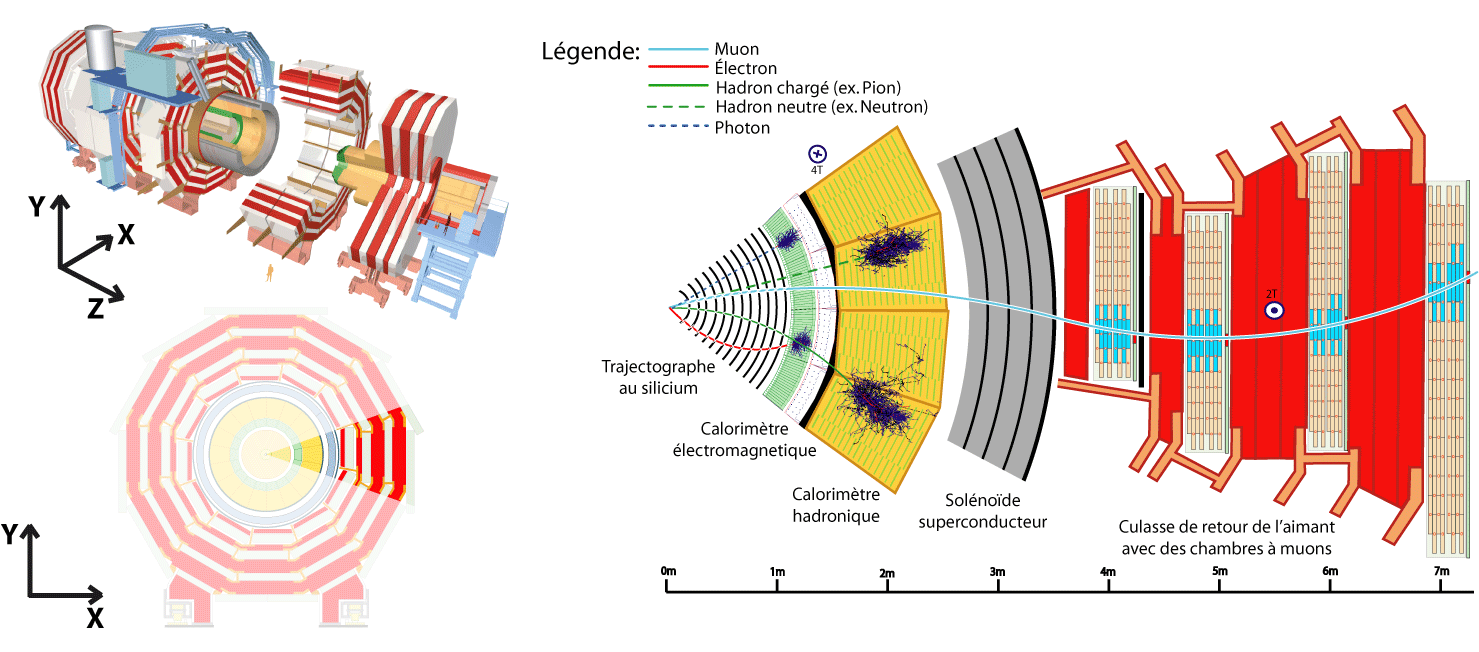
Physics objects are mainly reconstructed using methods like clustering and linking parts of a CMS subsystem to parts of other CMS subsystems. For instance, electromagnetic objects (electrons or photons) are reconstructed by the linking of tracks with ECAL energy deposits.

These actions are essential parts of the so-called Particle Flow (PF) algorithm.

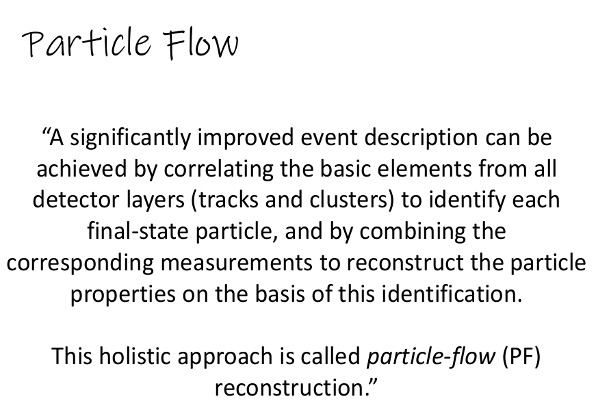
The particle-flow (PF) algorithm aims at reconstructing and identifying all stable particles in the event, i.e., electrons, muons, photons, charged hadrons and neutral hadrons, with a thorough combination of all CMS sub-detectors towards an optimal determination of their direction, energy and type. This list of individual particles is then used, as if it came from a Monte-Carlo event generator, to build jets (from which the quark and gluon energies and directions are inferred), to determine the missing transverse energy (which gives an estimate of the direction and energy of the neutrinos and other invisible particles), to reconstruct and identify taus from their decay products and more.

The PF algorith and all its reconstruction tributaries are written in C++ and are part of the CMSSW software.

The Physics Object Extractor Tool (POET)

The 2015 POET repository instructions read “… POET repository contains packages that verse instructions and examples on how to extract physics (objects) information from Run 2 (MiniAOD format) CMS open/legacy data and methods or tools needed for processing them”

POET was thought, originally, as tool to learn how to use CMSSW to access objects in an easier fashion. The code written by CMS experienced users could be extremely convoluted, but it all follows the same logic. POET tries to show how to do it in a pedagogical way by separating the processing of different objects. We will learn about this in this section.

POET is just a collection of CMSSW EDAnalyzers, very similar to the one your already worked with beforehand, the DemoAnalyzer.

We will learn about them in order to extract the information we need. We will focus on getting our code in shape so we can perform a simplified analysis using 2015 Run 2 data.

How to run with POET

Let us start with learning how to run with POET.

First, fire up your CMSSW Docker container already used during the pre-exercises.

docker start -i my_od #use the name you gave to yours

Once inside your container, make sure you are at the src directory level of your CMSSW area

pwd

/code/CMSSW_7_6_7/src

Let’s clone the POET brach that we will use for this lesson:

git clone -b odws2022-poetlesson https://github.com/cms-opendata-analyses/PhysObjectExtractorTool.git

Now, cd to the package of interest:

cd PhysObjectExtractorTool/PhysObjectExtractor/

Explore this directory with a ls command. You will notice it has a similar structure as the Demo/DemoAnalyzer package you already worked with.
Explore the src directory, you will find several EDAnalyzers (similar to the DemoAnalyzer.cc EDAnalyzer), essentially one for each object of interest.

ls src

ElectronAnalyzer.cc  GenParticleAnalyzer.cc  MetAnalyzer.cc   PhotonAnalyzer.cc     TauAnalyzer.cc          TriggerAnalyzer.cc
FatjetAnalyzer.cc    JetAnalyzer.cc          MuonAnalyzer.cc  SimpleEleMuFilter.cc  TriggObjectAnalyzer.cc  VertexAnalyzer.cc

Then, it is no surprise that you will find the configurator python file inside the python directory. There is just one configurator to configure anything that we want to do with POET. It is called poet_cfg.py. Open it from you host machine, using your favorite editor. This is what you will see:

import FWCore.ParameterSet.Config as cms
import FWCore.Utilities.FileUtils as FileUtils
import FWCore.PythonUtilities.LumiList as LumiList
import FWCore.ParameterSet.Types as CfgTypes
import sys

#---- sys.argv takes the parameters given as input cmsRun PhysObjectExtractor/python/poet_cfg.py <isData (default=False)>
#----  e.g: cmsRun PhysObjectExtractor/python/poet_cfg.py True
#---- NB the first two parameters are always "cmsRun" and the config file name
#---- Work with data (if False, assumed MC simulations)
#---- This needs to be in agreement with the input files/datasets below.
if len(sys.argv) > 2:
    isData = eval(sys.argv[2])
else:
    isData = False
isMC = True
if isData: isMC = False

process = cms.Process("POET")

#---- Configure the framework messaging system
#---- https://twiki.cern.ch/twiki/bin/view/CMSPublic/SWGuideMessageLogger
process.load("FWCore.MessageService.MessageLogger_cfi")
process.MessageLogger.cerr.threshold = "WARNING"
process.MessageLogger.categories.append("POET")
process.MessageLogger.cerr.INFO = cms.untracked.PSet(
    limit=cms.untracked.int32(-1))
process.options = cms.untracked.PSet(wantSummary=cms.untracked.bool(True))

#---- Select the maximum number of events to process (if -1, run over all events)
process.maxEvents = cms.untracked.PSet( input = cms.untracked.int32(100) )



#---- Define the test source files to be read using the xrootd protocol (root://), or local files (file:)
process.source = cms.Source("PoolSource", fileNames = cms.untracked.vstring(
        #'root://eospublic.cern.ch//eos/opendata/cms/mc/RunIIFall15MiniAODv2/DYJetsToLL_M-10to50_TuneCUETP8M1_13TeV-amcatnloFXFX-pythia8/MINIAODSIM/PU25nsData2015v1_76X_mcRun2_asymptotic_v12-v1/00000/0005EA25-8CB8-E511-A910-00266CF85DA0.root'   
        'root://eospublic.cern.ch//eos/opendata/cms/mc/RunIIFall15MiniAODv2/TT_TuneCUETP8M1_13TeV-powheg-pythia8/MINIAODSIM/PU25nsData2015v1_76X_mcRun2_asymptotic_v12_ext3-v1/00000/02837459-03C2-E511-8EA2-002590A887AC.root'
        )
)
if isData:
    process.source.fileNames = cms.untracked.vstring(
        #'root://eospublic.cern.ch//eos/opendata/cms/Run2015D/DoubleMuon/MINIAOD/16Dec2015-v1/10000/000913F7-E9A7-E511-A286-003048FFD79C.root'
	'root://eospublic.cern.ch//eos/opendata/cms/Run2015D/SingleElectron/MINIAOD/08Jun2016-v1/10000/001A703B-B52E-E611-BA13-0025905A60B6.root'
        )


#----- Configure POET analyzers -----#
process.myelectrons = cms.EDAnalyzer('ElectronAnalyzer', 
                                     electrons = cms.InputTag("slimmedElectrons"), 
                                     vertices=cms.InputTag("offlineSlimmedPrimaryVertices"))

process.mymuons = cms.EDAnalyzer('MuonAnalyzer', 
                                 muons = cms.InputTag("slimmedMuons"), 
                                 vertices=cms.InputTag("offlineSlimmedPrimaryVertices"))




#----- RUN THE JOB! -----#
process.TFileService = cms.Service("TFileService", fileName=cms.string("myoutput.root"))

if isData:
	process.p = cms.Path(process.myelectrons)
else:
	process.p = cms.Path(process.myelectrons)

You already saw, in the pre-exercises, many of the features present in a regular configuration file. The poet_cfg.py file has more modules, however. Let’s understand what they do.

The first addition you can see is the possibility of ingesting an argument from the user:

#---- sys.argv takes the parameters given as input cmsRun PhysObjectExtractor/python/poet_cfg.py <isData (default=False)>
#----  e.g: cmsRun PhysObjectExtractor/python/poet_cfg.py True
#---- NB the first two parameters are always "cmsRun" and the config file name
#---- Work with data (if False, assumed MC simulations)
#---- This needs to be in agreement with the input files/datasets below.
if len(sys.argv) > 2:
    isData = eval(sys.argv[2])
else:
    isData = False
isMC = True
if isData: isMC = False

process = cms.Process("POET")

This basically tells you that you have the option of choosing between running over collisions data (or just data) or over montecarlo (MC) simulations. If you don’t give any argument, the isMC will remain true, whereas if you pass a True boolean, then the isData switch will become active.

This will have a direct impact on the kind of input file the process.source module will end up picking up:

#---- Define the test source files to be read using the xrootd protocol (root://), or local files (file:)
process.source = cms.Source("PoolSource", fileNames = cms.untracked.vstring(
        #'root://eospublic.cern.ch//eos/opendata/cms/mc/RunIIFall15MiniAODv2/DYJetsToLL_M-10to50_TuneCUETP8M1_13TeV-amcatnloFXFX-pythia8/MINIAODSIM/PU25nsData2015v1_76X_mcRun2_asymptotic_v12-v1/00000/0005EA25-8CB8-E511-A910-00266CF85DA0.root'   
        'root://eospublic.cern.ch//eos/opendata/cms/mc/RunIIFall15MiniAODv2/TT_TuneCUETP8M1_13TeV-powheg-pythia8/MINIAODSIM/PU25nsData2015v1_76X_mcRun2_asymptotic_v12_ext3-v1/00000/02837459-03C2-E511-8EA2-002590A887AC.root'
        )
)
if isData:
    process.source.fileNames = cms.untracked.vstring(
        #'root://eospublic.cern.ch//eos/opendata/cms/Run2015D/DoubleMuon/MINIAOD/16Dec2015-v1/10000/000913F7-E9A7-E511-A286-003048FFD79C.root'
	'root://eospublic.cern.ch//eos/opendata/cms/Run2015D/SingleElectron/MINIAOD/08Jun2016-v1/10000/001A703B-B52E-E611-BA13-0025905A60B6.root'
        )

Let’s explore one of these input files. These are the data we release under the open data initiative. You notice from their name that their format is MINIAOD. A given dataset contains many of these files. Choose any you like and check its content, for instance:

edmDumpEventContent root://eospublic.cern.ch//eos/opendata/cms/mc/RunIIFall15MiniAODv2/TT_TuneCUETP8M1_13TeV-powheg-pythia8/MINIAODSIM/PU25nsData2015v1_76X_mcRun2_asymptotic_v12_ext3-v1/00000/02837459-03C2-E511-8EA2-002590A887AC.root

Type                                  Module                      Label             Process   
----------------------------------------------------------------------------------------------
LHEEventProduct                       "externalLHEProducer"       ""                "LHE"     
GenEventInfoProduct                   "generator"                 ""                "SIM"     
edm::TriggerResults                   "TriggerResults"            ""                "SIM"     
edm::TriggerResults                   "TriggerResults"            ""                "HLT"     
HcalNoiseSummary                      "hcalnoise"                 ""                "RECO"    
L1GlobalTriggerReadoutRecord          "gtDigis"                   ""                "RECO"    
double                                "fixedGridRhoAll"           ""                "RECO"    
double                                "fixedGridRhoFastjetAll"    ""                "RECO"    
double                                "fixedGridRhoFastjetAllCalo"   ""                "RECO"    
double                                "fixedGridRhoFastjetCentral"   ""                "RECO"    
double                                "fixedGridRhoFastjetCentralCalo"   ""                "RECO"    
double                                "fixedGridRhoFastjetCentralChargedPileUp"   ""                "RECO"    
double                                "fixedGridRhoFastjetCentralNeutral"   ""                "RECO"    
edm::TriggerResults                   "TriggerResults"            ""                "RECO"    
reco::BeamHaloSummary                 "BeamHaloSummary"           ""                "RECO"    
reco::BeamSpot                        "offlineBeamSpot"           ""                "RECO"    
vector<l1extra::L1EmParticle>         "l1extraParticles"          "Isolated"        "RECO"    
vector<l1extra::L1EmParticle>         "l1extraParticles"          "NonIsolated"     "RECO"    
vector<l1extra::L1EtMissParticle>     "l1extraParticles"          "MET"             "RECO"    
vector<l1extra::L1EtMissParticle>     "l1extraParticles"          "MHT"             "RECO"    
vector<l1extra::L1HFRings>            "l1extraParticles"          ""                "RECO"    
vector<l1extra::L1JetParticle>        "l1extraParticles"          "Central"         "RECO"    
vector<l1extra::L1JetParticle>        "l1extraParticles"          "Forward"         "RECO"    
vector<l1extra::L1JetParticle>        "l1extraParticles"          "IsoTau"          "RECO"    
vector<l1extra::L1JetParticle>        "l1extraParticles"          "Tau"             "RECO"    
vector<l1extra::L1MuonParticle>       "l1extraParticles"          ""                "RECO"    
edm::SortedCollection<EcalRecHit,edm::StrictWeakOrdering<EcalRecHit> >    "reducedEgamma"             "reducedEBRecHits"   "PAT"     
edm::SortedCollection<EcalRecHit,edm::StrictWeakOrdering<EcalRecHit> >    "reducedEgamma"             "reducedEERecHits"   "PAT"     
edm::SortedCollection<EcalRecHit,edm::StrictWeakOrdering<EcalRecHit> >    "reducedEgamma"             "reducedESRecHits"   "PAT"     
edm::TriggerResults                   "TriggerResults"            ""                "PAT"     
edm::ValueMap<float>                  "offlineSlimmedPrimaryVertices"   ""                "PAT"     
pat::PackedTriggerPrescales           "patTrigger"                ""                "PAT"     
pat::PackedTriggerPrescales           "patTrigger"                "l1max"           "PAT"     
pat::PackedTriggerPrescales           "patTrigger"                "l1min"           "PAT"     
vector<PileupSummaryInfo>             "slimmedAddPileupInfo"      ""                "PAT"     
vector<pat::Electron>                 "slimmedElectrons"          ""                "PAT"     
vector<pat::Jet>                      "slimmedJets"               ""                "PAT"     
vector<pat::Jet>                      "slimmedJetsAK8"            ""                "PAT"     
vector<pat::Jet>                      "slimmedJetsPuppi"          ""                "PAT"     
vector<pat::Jet>                      "slimmedJetsAK8PFCHSSoftDropPacked"   "SubJets"         "PAT"     
vector<pat::Jet>                      "slimmedJetsCMSTopTagCHSPacked"   "SubJets"         "PAT"     
vector<pat::MET>                      "slimmedMETs"               ""                "PAT"     
vector<pat::MET>                      "slimmedMETsPuppi"          ""                "PAT"     
vector<pat::Muon>                     "slimmedMuons"              ""                "PAT"     
vector<pat::PackedCandidate>          "lostTracks"                ""                "PAT"     
vector<pat::PackedCandidate>          "packedPFCandidates"        ""                "PAT"     
vector<pat::PackedGenParticle>        "packedGenParticles"        ""                "PAT"     
vector<pat::Photon>                   "slimmedPhotons"            ""                "PAT"     
vector<pat::Tau>                      "slimmedTaus"               ""                "PAT"     
vector<pat::TriggerObjectStandAlone>    "selectedPatTrigger"        ""                "PAT"     
vector<reco::CATopJetTagInfo>         "caTopTagInfosPAT"          ""                "PAT"     
vector<reco::CaloCluster>             "reducedEgamma"             "reducedEBEEClusters"   "PAT"     
vector<reco::CaloCluster>             "reducedEgamma"             "reducedESClusters"   "PAT"     
vector<reco::Conversion>              "reducedEgamma"             "reducedConversions"   "PAT"     
vector<reco::Conversion>              "reducedEgamma"             "reducedSingleLegConversions"   "PAT"     
vector<reco::GenJet>                  "slimmedGenJets"            ""                "PAT"     
vector<reco::GenJet>                  "slimmedGenJetsAK8"         ""                "PAT"     
vector<reco::GenParticle>             "prunedGenParticles"        ""                "PAT"     
vector<reco::GsfElectronCore>         "reducedEgamma"             "reducedGedGsfElectronCores"   "PAT"     
vector<reco::PhotonCore>              "reducedEgamma"             "reducedGedPhotonCores"   "PAT"     
vector<reco::SuperCluster>            "reducedEgamma"             "reducedSuperClusters"   "PAT"     
vector<reco::Vertex>                  "offlineSlimmedPrimaryVertices"   ""                "PAT"     
vector<reco::VertexCompositePtrCandidate>    "slimmedSecondaryVertices"   ""                "PAT"

This is essentially all the information you can get from MINIAOD files like this one. Put special attention to the anything related to Electron(s) or Muon(s). One thing you notice is that the acronym PAT is repeated several times. PAT stands for Physics Analysis Tool and is a framework within CMSSW that is extensively used to refine the selection of physical objects in CMS. The RECO variables are, however, lower level variables. There are also some objects that will give you additional information, like the HLT TriggerResults, which we will cover tomorrow.

Next in the poet_cfg.py file, you will find a couple of modules that are evidently associated to EDAnalyzers that deal with electrons and muons:

#----- Configure POET analyzers -----#
process.myelectrons = cms.EDAnalyzer('ElectronAnalyzer', 
                                     electrons = cms.InputTag("slimmedElectrons"), 
                                     vertices=cms.InputTag("offlineSlimmedPrimaryVertices"))

process.mymuons = cms.EDAnalyzer('MuonAnalyzer', 
                                 muons = cms.InputTag("slimmedMuons"), 
                                 vertices=cms.InputTag("offlineSlimmedPrimaryVertices"))

Remember, the construction cms.EDAnalyzer('ElectronAnalyzer', for instance, automatically tells you that there must be an EDAnalyzer called ElectronAnalyzer somewhere in this package. Indeed, if you list your src directory, you will find, among other EDAnalyzers (including the muon one), an ElectronAnalyzer.cc file. So, this module process.myelectrons configures that C++ code. Something similar is true for the MuonAnalyzer. Also notice that InputTags used in these modules correspond to the collections seen above when we dump the structure of the input file.

Finally, among the new features present in poet_cfg.py, there is a TFileService module. It is rather obvious that it will output a ROOT file called myoutput.root, which will most certainly contain the information that a given EDAnalyzer is spitting out.

process.TFileService = cms.Service("TFileService", fileName=cms.string("myoutput.root"))

Enough talk, let’s run POET!

Compile the code with scram b and then run POET twice with the True argument:

• First with cmsRun python/poet_cfg.py True
• and then with just cmsRun python/poet_cfg.py (without the True boolean, so we run over MC simulations)

Open the myoutput.root file that gets produced and have a quick look with the TBrowser.

You will notice that only electron variables got stored. Can you fix the poet_cfg.py so we get the information from muons as well?

Solution

Just add the process.mymuons module to the running paths at the end of the config file. Don’t forget the + sign. Run it again and check if you get some muon info (you don’t need to recompile, that is the beauty of config files).

That is the way in which we can add different objects to our output file. We will look at the C++ code of some of these objects and think a little bit about the physics involed. We will defer that for the next episodes in this lesson, however.

Adding data quality to the configuration

The detector is not perfect and sometimes there is a high voltage source that peaks or surges, for instance, and with it many channels of a given subdetector. When that – or any other problem – happens, the DOC (Detector on-call expert) for that subsystem is called, the run is generally stopped and the problem is fixed. However, a few lumi sections (LS), containing some events, may need to be discarted (you don’t want something that can fake an exotic particle due to a sensor spiking, for example).

There is a tremendous effort by many people in the collaboration to assure the quality of our data. We do this by keeping record of only the good LS in a json file. For convinience, we have put this file in the data directory of the POET repository. More information can be found here.

Add data qualtiy to POET

In order to filter out those bad LS we need to add a special module to our poet_cfg.py file. Follow the cues in the snippet below at place at the right location within the poet_cfg.py file and save it (in general the order of modules hardly matter for CMSSW config files; this one is an exception). Run the configuration again to make sure nothing breaks. It is possible that you don’t see anything chaning due to very few events we are running with (100).

#---- Apply the data quality JSON file filter. This example is for 2015 data
#---- It needs to be done after the process.source definition
#---- Make sure the location of the file agrees with your setup
goodJSON = "data/Cert_13TeV_16Dec2015ReReco_Collisions15_25ns_JSON_v2.txt"
myLumis = LumiList.LumiList(filename=goodJSON).getCMSSWString().split(",")
process.source.lumisToProcess = CfgTypes.untracked(CfgTypes.VLuminosityBlockRange())
process.source.lumisToProcess.extend(myLumis) 

Add a new physics object to the configuration

You can see in the src directory that there is already code for many other objects, not just electrons or muons. Some of these EDAnalyzers are complete while others are still being developed.

Adding primary vertices

For this next task your job is to add primary vertices to our myoutput.root file. Plese resist the urge to look at the answer. Only use it to compare your attempt

As you may have noticed, there is already code written for this. You can find it under src/VertexAnalyzer.cc. One can explore this code and figure out how to configure it by checking out its constructor.

As a hint, know that the beamspot is the the luminous region produced by the collisions of proton beams. It is basically the true place where the main collisions took place, which is not necessarily the center of the detector.

The configuration should look really similar to the electron or muon modules. Also, note that the InputTag should match the collections available in the input file, whose information we dumped above.

Make this addition to the poet_config.py file as a process.mypvertex module and do not forget to add it to both of the final paths. Run the new configuration and make sure the mypvertex branch is added to the file.

Solution

Somewhere before the final paths in the poet_config.py you should have added:

process.mypvertex = cms.EDAnalyzer('VertexAnalyzer',
                                   vertices=cms.InputTag("offlineSlimmedPrimaryVertices"), 
                                   beams=cms.InputTag("offlineBeamSpot"))

Also, you need to add this module to the final paths:

if isData:
	process.p = cms.Path(process.myelectrons + process.mymuons + process.mypvertex)
else:
	process.p = cms.Path(process.myelectrons + process.mymuons + process.mypvertex)

Common treatment of physics objects

If you look briefly at the different EDAnalyzers in the src directory you will notice they share the code structure. One could build a specific analyzer in order to access the information from a particular type. A summary of the high level physics objects can be found in this Twiki page from CMS.

POET structure of EDAnalyzers

During your prep-work, you already saw the main structure of an EDAnalyzer. We have added certain functionalities, which we briefly present here using the src/ElectronAnalyzer.cc as an example.

The first thing to to notice is that all the EDAnalyzers in POET book a ROOT TTree and some variables in the class definition to store the physics objects information:

      TTree *mtree;
      int numelectron; //number of electrons in the event
      std::vector<float> electron_e;
      std::vector<float> electron_pt;
      std::vector<float> electron_px;
      std::vector<float> electron_py;
      std::vector<float> electron_pz;
      std::vector<float> electron_eta;
      std::vector<float> electron_phi;

In the constructor, a TFileService object is used to deal with the final ROOT output file and some ROOT braches are specified. Of course, these are the ones which appear in the myoutput.root file.

   edm::Service<TFileService> fs;
   mtree = fs->make<TTree>("Events", "Events");
  
  mtree->Branch("numberelectron",&numelectron);   
  mtree->GetBranch("numberelectron")->SetTitle("number of electrons");
  mtree->Branch("electron_e",&electron_e);
  mtree->GetBranch("electron_e")->SetTitle("electron energy");
  mtree->Branch("electron_pt",&electron_pt);
  mtree->GetBranch("electron_pt")->SetTitle("electron transverse momentum");
  mtree->Branch("electron_px",&electron_px);
  mtree->GetBranch("electron_px")->SetTitle("electron momentum x-component");
  mtree->Branch("electron_py",&electron_py);
  mtree->GetBranch("electron_py")->SetTitle("electron momentum y-component");
  mtree->Branch("electron_pz",&electron_pz);
  mtree->GetBranch("electron_pz")->SetTitle("electron momentum z-component");
  mtree->Branch("electron_eta",&electron_eta);
  mtree->GetBranch("electron_eta")->SetTitle("electron pseudorapidity");
  mtree->Branch("electron_phi",&electron_phi);
  mtree->GetBranch("electron_phi")->SetTitle("electron polar angle");

Essentially all of the EDAnalyzers clear the variable containers and loop over the objects present in the event.

Finally, many of the most important kinematic quantities defining a physics object are accessed in a common way across all the objects. Most objects have associated energy-momentum vectors, typically constructed using transverse momentum, pseudorapdity, azimuthal angle, and mass or energy.

   numelectron = 0;
   electron_e.clear();
   electron_pt.clear();
   electron_px.clear();
   electron_py.clear();
   electron_pz.clear();
   electron_eta.clear();
   electron_phi.clear();
   electron_ch.clear();
   electron_iso.clear();
   electron_veto.clear();//
   electron_isLoose.clear();
   electron_isMedium.clear();
   electron_isTight.clear();
   electron_dxy.clear();
   electron_dz.clear();
   electron_dxyError.clear();
   electron_dzError.clear();
   electron_ismvaLoose.clear();
   electron_ismvaTight.clear();

    for (const pat::Electron &el : *electrons)
    {
      electron_e.push_back(el.energy());
      electron_pt.push_back(el.pt());
      electron_px.push_back(el.px());
      electron_py.push_back(el.py());
      electron_pz.push_back(el.pz());
      electron_eta.push_back(el.eta());
      electron_phi.push_back(el.phi());

Final config file from this episode

At the end of this episode, your configuration file should look something like the one below. We will pick up from here in the next episode.

View final file

import FWCore.ParameterSet.Config as cms
import FWCore.Utilities.FileUtils as FileUtils
import FWCore.PythonUtilities.LumiList as LumiList
import FWCore.ParameterSet.Types as CfgTypes
import sys

#---- sys.argv takes the parameters given as input cmsRun PhysObjectExtractor/python/poet_cfg.py <isData (default=False)>
#----  e.g: cmsRun PhysObjectExtractor/python/poet_cfg.py True
#---- NB the first two parameters are always "cmsRun" and the config file name
#---- Work with data (if False, assumed MC simulations)
#---- This needs to be in agreement with the input files/datasets below.
if len(sys.argv) > 2:
    isData = eval(sys.argv[2])
else:
    isData = False
isMC = True
if isData: isMC = False

process = cms.Process("POET")

#---- Configure the framework messaging system
#---- https://twiki.cern.ch/twiki/bin/view/CMSPublic/SWGuideMessageLogger
process.load("FWCore.MessageService.MessageLogger_cfi")
process.MessageLogger.cerr.threshold = "WARNING"
process.MessageLogger.categories.append("POET")
process.MessageLogger.cerr.INFO = cms.untracked.PSet(
    limit=cms.untracked.int32(-1))
process.options = cms.untracked.PSet(wantSummary=cms.untracked.bool(True))

#---- Select the maximum number of events to process (if -1, run over all events)
process.maxEvents = cms.untracked.PSet( input = cms.untracked.int32(100) )



#---- Define the test source files to be read using the xrootd protocol (root://), or local files (file:)
process.source = cms.Source("PoolSource", fileNames = cms.untracked.vstring(
        #'root://eospublic.cern.ch//eos/opendata/cms/mc/RunIIFall15MiniAODv2/DYJetsToLL_M-10to50_TuneCUETP8M1_13TeV-amcatnloFXFX-pythia8/MINIAODSIM/PU25nsData2015v1_76X_mcRun2_asymptotic_v12-v1/00000/0005EA25-8CB8-E511-A910-00266CF85DA0.root'   
        'root://eospublic.cern.ch//eos/opendata/cms/mc/RunIIFall15MiniAODv2/TT_TuneCUETP8M1_13TeV-powheg-pythia8/MINIAODSIM/PU25nsData2015v1_76X_mcRun2_asymptotic_v12_ext3-v1/00000/02837459-03C2-E511-8EA2-002590A887AC.root'
        )
)
if isData:
    process.source.fileNames = cms.untracked.vstring(
        #'root://eospublic.cern.ch//eos/opendata/cms/Run2015D/DoubleMuon/MINIAOD/16Dec2015-v1/10000/000913F7-E9A7-E511-A286-003048FFD79C.root'
	'root://eospublic.cern.ch//eos/opendata/cms/Run2015D/SingleElectron/MINIAOD/08Jun2016-v1/10000/001A703B-B52E-E611-BA13-0025905A60B6.root'
        )


#---- Apply the data quality JSON file filter. This example is for 2015 data
#---- It needs to be done after the process.source definition
#---- Make sure the location of the file agrees with your setup
goodJSON = "data/Cert_13TeV_16Dec2015ReReco_Collisions15_25ns_JSON_v2.txt"
myLumis = LumiList.LumiList(filename=goodJSON).getCMSSWString().split(",")
process.source.lumisToProcess = CfgTypes.untracked(CfgTypes.VLuminosityBlockRange())
process.source.lumisToProcess.extend(myLumis) 



#----- Configure POET analyzers -----#
process.myelectrons = cms.EDAnalyzer('ElectronAnalyzer', 
                                     electrons = cms.InputTag("slimmedElectrons"), 
                                     vertices=cms.InputTag("offlineSlimmedPrimaryVertices"))

process.mymuons = cms.EDAnalyzer('MuonAnalyzer', 
                                 muons = cms.InputTag("slimmedMuons"), 
                                 vertices=cms.InputTag("offlineSlimmedPrimaryVertices"))

process.mypvertex = cms.EDAnalyzer('VertexAnalyzer',
                                   vertices=cms.InputTag("offlineSlimmedPrimaryVertices"), 
                                   beams=cms.InputTag("offlineBeamSpot"))




#----- RUN THE JOB! -----#
process.TFileService = cms.Service("TFileService", fileName=cms.string("myoutput.root"))

if isData:
	process.p = cms.Path(process.myelectrons + process.mymuons + process.mypvertex)
else:
	process.p = cms.Path(process.myelectrons + process.mymuons + process.mypvertex)

Key Points

• Physics objects are the final abstraction in the detector that can be associated to physical entities like particles.

• POET is a collection of CMSSW EDAnalyzers meant to teach how to access physics objects information.

Electrons

Overview

Teaching: 10 min
Exercises: 30 min

Questions

• What are electromagnetic objects

• How are electrons treated in CMS?

• What variable are available using POET?

• How can one add a new electron variable?

Objectives

• Understand what electromagnetic objects are in CMS

• Learn electron member functions for common track-based quantities

• Learn member functions for identification and isolation of electrons

• Learn member functions for electron detector-related quantities

• Learn how to add new information to the EDAnalyzer

Prerequisites

• We will be still running on the CMSSW Docker container. If you closed it for some reason, just fire it back up.
• During the last episode we made modifications to our python/poet_cfg.py file. If for some reason yours got into an invalid state, just copy/paste from the last episode.

Motivation

At the equator of the workshop we will be working on the main activity, which is to attempt to replicate a CMS physics analysis in a simplified way using modern analysis tools. The final state that we will be looking at contains electrons, muons and jets. We are using these objects as examples to review the way in which we extract physics objects information.

The analysis requires some special variables, which we will have to figure out how to implement.

Electromagnetic objects

We call photons and electrons electromagnetic particles because they leave most of their energy in the electromagnetic calorimeter (ECAL) so they share many common properties and functions

Many of the different hypothetical exotic particles are unstable and can transform, or decay, into electrons, photons, or both. Electrons and photons are also standard tools to measure better and understand the properties of already known particles. For example, one way to find a Higgs Boson is by looking for signs of two photons, or four electrons in the debris of high energy collisions. Because electrons and photons are crucial in so many different scenarios, the physicists in the CMS collaboration make sure to do their best to reconstruct and identify these objects.

As depicted in the figure above, tracks – from the pixel and silicon tracker systems – as well as ECAL energy deposits are used to identify the passage of electrons in CMS. Being charged, electron trajectories curve inside the CMS magnetic field. Photons are similar objects but with no tracks. Sophisticated algorithms are run in the reconstruction to take into account subtleties related to the identification of an electromagnetic particle. An example is the convoluted showering of sub-photons and sub-electrons that can reach the ECAL due to bremsstrahlung and photon conversions.

We measure momentum and energy but also other properties of these objects that help analysts understand better their quality and origin. Let’s explore the ElectronAnalyzer in POET to get a sense of some of these properties.

The ElectronAnalyzer.cc EDAnalyzer

Fire up your favorite editor on your local machine and open the src/ElectronAnalyzer.cc file from the PhysObjectExtractorTool/PhysObjectExtractor package of your curent POET repository.

Needed libraries

The first thing that you will see is a set of includes. In particular we have a set of headers for electrons:

...
//class to extract electron information
#include "DataFormats/PatCandidates/interface/Electron.h"
#include "DataFormats/EgammaCandidates/interface/GsfElectron.h"
#include "DataFormats/VertexReco/interface/VertexFwd.h"
#include "DataFormats/VertexReco/interface/Vertex.h"
...

Electron 4-vector and track information

In the loop over the electron collection in ElectronAnalyzer.cc, we access elements of the four-vector as shown in the last episode:

for (const pat::Electron &el : *electrons){
    ...
    electron_e.push_back(el.energy());
    electron_pt.push_back(el.pt());
    ...
}

Most charged physics objects are also connected to tracks from the CMS tracking detectors. The charge of the object can be queried directly:

electron_ch.push_back(el.charge());

Information from tracks provides other kinematic quantities that are common to multiple types of objects. Often, the most pertinent information about an object to access from its associated track is its impact parameter with respect to the primary interaction vertex. We can access the impact parameters in the xy-plane (dxy or d0) and along the beam axis (dz), as well as their respective uncertainties.

math::XYZPoint pv(vertices->begin()->position());
...

electron_dxy.push_back(el.gsfTrack()->dxy(pv));
electron_dz.push_back(el.gsfTrack()->dz(pv));
electron_dxyError.push_back(el.gsfTrack()->d0Error());
electron_dzError.push_back(el.gsfTrack()->dzError());

Note: in the case of Photons, since they are neutral objects, they do not have a direct track link (though displaced track segments may appear from electrons or positrons produced by the photon as it transits the detector material). While the charge() method exists for all objects, it is not used in photon analyses.

Detector information for identification

The most signicant difference between a list of certain particles from a Monte Carlo generator and a list of the corresponding physics objects from CMS is likely the inherent uncertainty in the reconstruction. Selection of “a muon” or “an electron” for analysis requires algorithms designed to separate “real” objects from “fakes”. These are called identification algorithms.

Other algorithms are designed to measure the amount of energy deposited near the object, to determine if it was likely produced near the primary interaction (typically little nearby energy), or from the decay of a longer-lived particle (typically a lot of nearby energy). These are called isolation algorithms. Many types of isolation algorithms exist to deal with unique physics cases!

Both types of algorithms function using working points that are described on a spectrum from “loose” to “tight”. Working points that are “looser” tend to have a high efficiency for accepting real objects, but perhaps a poor rejection rate for “fake” objects. Working points that are “tighter” tend to have lower efficiencies for accepting real objects, but much better rejection rates for “fake” objects. The choice of working point is highly analysis dependent! Some analyses value efficiency over background rejection, and some analyses are the opposite.

The standard identification and isolation algorithm results can be accessed from the physics object classes.

Multivariate Electron Identification (MVA)

In the Multi-variate Analysis (MVA) approach, one forms a single discriminator variable that is computed based on multiple parameters of the electron object and provides the best separation between the signal and backgrounds by means of multivariate analysis methods and statistical learning tools. One can then cut on discriminator value or use the distribution of the values for a shape based statistical analysis.

There are two basic types of MVAs that are usually provided:

• the triggering MVA: the discriminator is trained on the electrons that pass typical electron trigger requirements
• the non-triggering MVA: the discriminator is trained on all electrons regardless of the trigger

As an example in the ElectronAnalyzer we use the non-triggering MVA. Note that the tags used are ...wp90 and ...wp80. As mentioned above, the difference lies on the working point (wp). Both 80% and 90% are the signal efficiency for each MVA category as measured on electron.

      electron_ismvaLoose.push_back(el.electronID("mvaEleID-Spring15-25ns-nonTrig-V1-wp90"));
      electron_ismvaTight.push_back(el.electronID("mvaEleID-Spring15-25ns-nonTrig-V1-wp80"));

The MVA training provides working points with decreased electron fake rate.

Cut Based Electron ID

Most pat::<object> classes contain member functions that return detector-related information. In the case of electrons, we see this information used as identification criteria:

...
      electron_veto.push_back(el.electronID("cutBasedElectronID-Spring15-25ns-V1-standalone-veto"));//
      electron_isLoose.push_back(el.electronID("cutBasedElectronID-Spring15-25ns-V1-standalone-loose"));
      electron_isMedium.push_back(el.electronID("cutBasedElectronID-Spring15-25ns-V1-standalone-medium"));
      electron_isTight.push_back(el.electronID("cutBasedElectronID-Spring15-25ns-V1-standalone-tight"));
...

Let’s break down these criteria:

• cutBasedElectronID...veto is a tag that rejects electrons coming from photon conversions in the tracker, which should instead be reconstructed as part of the photon.

Four standard working points are provided

• Veto (average efficiency ~95%). Use this working point for third lepton veto or counting.
• Loose (average efficiency ~90%). Use this working point when backgrounds are rather low.
• Medium (average efficiency ~80%). This is a good starting point for generic measurements involving W or Z bosons.
• Tight (average efficiency ~70%). Use this working point for measurements where backgrounds are a serious problem.

Isolation is computed in similar ways for all physics objects: search for particles in a cone around the object of interest and sum up their energies, subtracting off the energy deposited by pileup particles. This sum divided by the object of interest’s transverse momentum is called relative isolation and is the most common way to determine whether an object was produced “promptly” in or following the proton-proton collision (ex: electrons from a Z boson decay, or photons from a Higgs boson decay). Relative isolation values will tend to be large for particles that emerged from weak decays of hadrons within jets, or other similar “nonprompt” processes. For electrons, isolation is computed as:

...
electron_iso.push_back(el.ecalPFClusterIso());
...

Note: these POET implementations of identification working points are appropriate for 2015 data analysis.

Adding the sip3d variable for electrons

If you read the article mentioned above, which we would like to partially reproduce, you would encounter the usage of a variable which is described as:

Nonprompt leptons that come from the decays of long-lived hadrons are rejected by requiring that the significance of the three-dimensional (3D) impact parameter of the lepton track, relative to the primary event vertex, is less than four standard deviations. This requirement effectively reduces the contamination from multijet events, while keeping a high efficiency for the signal

Can you find this (spi3d) variable in the ElectronAnalyzer code? … Well, if you couldn’t it is because we do not have it (yet).

As it turns out, implementing the ip3d variable is very simple because it is already availabe as an accessible method in the class we use to access basically everything.
However, its partner sip3d is not.

Your task will be to implement this variable into the ElectronAnalyzer.cc so we can use it later in our simplified analysis replica.

A few hints:

• There is an alternative way of accesing this ip3d variable, as you can see here. We would be, essentially, recomputing this variable out of transient tracks. We can build transient tracks from our electron’s track, which is easily accessible as you could note here.
• What the code snippet above tells us is that the significance should come from an C++ object created by the IPTools class.
• Exploring that class you will find the appropriate C++ object and how to retrieve it.
• The C++ object name will naturally point you to the class to look at in the header of the IPTools class. Once you find it, you will be able to identify the needed method for extracting the significance.
• You just need to digest all this information and implement it in the ElectronAnalyzer.cc.
• Do not forget to add the TransientTrack and IPTools libraries to the BuildFile.xml of the package and recompile your code.
• Important note: transient tracks are built with information from the conditions database of the experiment and info about the magnetic field and geometry. Therefore, to make your life a bit easier, we plainly ask you to include these lines in your poet_cfg.py file so you can have access to this information. No more changes are needed in the config file.

#---- Needed configuration for dealing with transient tracks if required
process.load("TrackingTools/TransientTrack/TransientTrackBuilder_cfi")
process.load("Configuration.Geometry.GeometryIdeal_cff")
process.load("Configuration.StandardSequences.MagneticField_cff")

#---- These two lines are needed if you require access to the conditions database. E.g., to get jet energy corrections, trigger prescales, etc.
process.load('Configuration.StandardSequences.Services_cff')
process.load('Configuration.StandardSequences.FrontierConditions_GlobalTag_cff')
#---- If the container has local DB files available, uncomment lines like the ones below instead of the corresponding lines above
if isData: process.GlobalTag.connect = cms.string('sqlite_file:/cvmfs/cms-opendata-conddb.cern.ch/76X_dataRun2_16Dec2015_v0.db')
else: process.GlobalTag.connect = cms.string('sqlite_file:/cvmfs/cms-opendata-conddb.cern.ch/76X_mcRun2_asymptotic_RunIIFall15DR76_v1.db')
#---- The global tag must correspond to the needed epoch (comment out if no conditions needed)
if isData: process.GlobalTag.globaltag = '76X_dataRun2_16Dec2015_v0'
else: process.GlobalTag.globaltag = "76X_mcRun2_asymptotic_RunIIFall15DR76_v1"

Solution:

We will add two variables. Let’s see:

The required std vector variables are the following:

std::vector<double> electron_ip3d;	
std::vector<double> electron_sip3d;

The mtree variables could look like these:

mtree->Branch("electron_ip3d",&electron_ip3d);
mtree->GetBranch("electron_ip3d")->SetTitle("electron impact parameter in 3d");
mtree->Branch("electron_sip3d",&electron_sip3d);
mtree->GetBranch("electron_sip3d")->SetTitle("electron significance on impact parameter in 3d");

Note that mtree stores the information in each variable.

Vector clearing:

electron_ip3d.clear();
electron_sip3d.clear();

and finally almost at the bottom of the electron loop:

...
electron_ismvaTight.push_back(el.electronID("mvaEleID-Spring15-25ns-nonTrig-V1-wp80"));

edm::ESHandle<TransientTrackBuilder> trackBuilder;
iSetup.get<TransientTrackRecord>().get("TransientTrackBuilder", trackBuilder);
reco::TransientTrack tt = trackBuilder->build(el.gsfTrack());
std::pair<bool,Measurement1D> ip3dpv = IPTools::absoluteImpactParameter3D(tt, primaryVertex);
electron_ip3d.push_back(ip3dpv.second.value());
electron_sip3d.push_back(ip3dpv.second.significance());

numelectron++;
...

Here are the files with the implemented solution. We will pick up from here at the start of the Muons episode after the break.

• Download this file and save it as python/poet_cfg.py
• Download this file and save it as src/ElectronAnalyzer.cc
• Download this file and save it as BuildFile.xml

Key Points

• Quantities such as impact parameters and charge have common member functions.

• Physics objects in CMS are reconstructed from detector signals and are never 100% certain!

• Identification and isolation algorithms are important for reducing fake objects.

• One can add additional informtion to the EDAnalyzer

Break

Overview

Teaching: 0 min
Exercises: 30 min

Questions

• Which type of coffee will you drink on your break?

Objectives

• Acquire coffee. Drink coffee.

Key Points

• Any type of coffee is refreshing after so much concentrated learning.

Muons

Overview

Teaching: 10 min
Exercises: 30 min

Questions

• How are muons reconstructed in CMS?

• How are muons treated in CMS OpenData?

• How do I add variables to the muon analyzer?

Objectives

• Understand how muons are reconstructed in CMS

• Learn member functions for muon track-based quantities

• Learn member functions for identification and isolation of muons

• Learn how to add new variables to the muon analyzer

Prerequisites

• We will be still running on the CMSSW Docker container. If you closed it for some reason, just fire it back up.
• During the last episode we made modifications to a few files. If you fell behind, worry not, you can get the modifications with the files below:
  • Download this file and save it as python/poet_cfg.py
  • Download this file and save it as src/ElectronAnalyzer.cc
  • Download this file and save it as BuildFile.xml

Overview of muon reconstruction

Muons are the M in CMS (Compact Muon Solenoid). This is in part because they are reconstructed basically using all the CMS sub-detectors. As it nicely summarized here:

[A muon] is measured by fitting a curve to the hits registered in the four muon stations, which are located outside of the magnet coil, interleaved with iron “return yoke” plates. The particle path is measured by tracking its position through the multiple active layers of each station; for improved precision, this information is combined with the CMS silicon tracker measurements. Measuring the trajectory provides a measurement of particle momentum. Indeed, the strong magnetic field generated by the CMS solenoid bends the particle’s trajectory, with a bending radius that depends on its momentum: the more straight the track, the higher the momentum.

Depending essentially on the kind of sub-detectors were used to reconstruct muons, they are usually classified accroding to the summary image below.

Muons have many features in common with electrons, but their own unique identification algorithms. We will be studying the MuonAnalyzer.cc, which is part of the POET collection of EDAnalyzers.

The MuonAnalyzer.cc EDAnalyzer

If you open the src/MuonAnalyzer.cc file, you will notice the headers used to extract information for Muons. As for the electron, you may have noticed that several variables depend also on (or are calculated with respect to) the primary vertex.

#include "DataFormats/PatCandidates/interface/Muon.h"
#include "DataFormats/VertexReco/interface/VertexFwd.h"
#include "DataFormats/VertexReco/interface/Vertex.h"

Now, remember the EDAnalyzer class you learned about in the pre-exercises and how to access data inside the EDAnalyzer. The analyze function of an EDAnalyzer is performed once per event. Muons can be accessed like this:

void
MuonAnalyzer::analyze(const edm::Event &iEvent, const edm::EventSetup &iSetup)
{

  using namespace edm;
  using namespace std;

  Handle<pat::MuonCollection> muons;
  iEvent.getByToken(muonToken_, muons);

  Handle<reco::VertexCollection> vertices;
  iEvent.getByToken(vtxToken_, vertices);

The result of the getToken method is an object called “muons”, which is a collection of all the muon objects. Collection classes are generally constructed as vectors. We can quickly create a loop to access individual muons:

for (const pat::Muon &mu : *muons){
  {

    muon_e.push_back(mu.energy());
    muon_pt.push_back(mu.pt());
    muon_eta.push_back(mu.eta());
    muon_phi.push_back(mu.phi());

    muon_px.push_back(mu.px());
    muon_py.push_back(mu.py());
    muon_pz.push_back(mu.pz());

}

Many of the most important kinematic quantities defining a physics object are accessed in a common way across all the objects. They have associated energy-momentum vectors, typically constructed using transverse momentum, pseudorapdity, azimuthal angle, and mass or energy. In our case of study, the MuonAnalyzer.cc, the muon four-vector elements are accessed as shown above.

Muon identification and isolation

To get information associated to the track of the muon, we have to include specific variables. Those variables are added inside the private member function, as vector variables. The primary purpose is to record several values.

std::vector<float> muon_dxy;
std::vector<float> muon_dz;
std::vector<float> muon_dxyError;
std::vector<float> muon_dzError;

The process for accesing the track includes a loop which is placed in the analyzer function MuonAnalyzer::MuonAnalyzer, as the previous example.

for (const pat::Muon &mu : *muons)
    { muon_dxy.push_back(mu.muonBestTrack()->dxy(PV.position()));
      muon_dz.push_back(mu.muonBestTrack()->dz(PV.position()));
      muon_dxyError.push_back(mu.muonBestTrack()->d0Error());
      muon_dzError.push_back(mu.muonBestTrack()->dzError());
}

For initializing the variables, one has to clear them at the beginning of the analyzer function:

muon_dxy.clear();
muon_dz.clear();
muon_dxyError.clear();
muon_dzError.clear();

The CMS Muon object group has created member functions for the identification algorithms that store pass/fail decisions about the quality of each muon. As shown below, the algorithm depends on which vertex is considered as the primary interaction vertex.

Hard processes produce large angles between the final state partons. The final object of interest will be separated from the other objects in the event or be isolated. For instance, an isolated muon might be produced in the decay of a W boson. In contrast, a non-isolated muon can come from a weak decay inside a jet.

Muon isolation is calculated from a combination of factors: energy from charged hadrons, energy from neutral hadrons, and energy from photons, all in a cone of radius \(R = \sqrt{\eta^2 + \phi^2} < 0.3\) or \(<0.4\) around the muon. Many algorithms also feature a correction factor that subtracts average energy expected from pileup contributions to this cone – we’ll explore this later as an exercise. Decisions are made by comparing this energy sum to the transverse momentum of the muon.

auto iso04 = mu.pfIsolationR04();
muon_pfreliso04all.push_back((iso04.sumChargedHadronPt + iso04.sumNeutralHadronEt + iso04.sumPhotonEt)/mu.pt());

Modifications to align with our target analysis

For muons, we will also need the sip3d variable we included already for the electrons. This is the next task:

Add the sip3d variable to muons

Now that you know the answer for electrons, it should be rather straight-forward to implent something similar for the muon analyzer. Go ahead and make that change very quickly. Don’t forget to recompile and test. Make sure the myoutput.root histogram contains this variable for muons as well as for electrons.

Solution

You can download this file and save it as src/MuonAnalyzer.cc. Do not forget to recompile and run.

Now, there is another variable that was used for our target analysis but doesn’t exist in your src/MuonAnalyzer.cc.

Muon isolation is based on the sum of the \(p_{T}\) of the charged and neutral hadrons as well as photons reconstructed in a cone R=0.4 around the muon momentum. The sum of the \(p_{T}\) of the charged hadrons associated to vertices other than the primary vertex, is used to correct for pileup contamination in the total flux of neutrals found in the muon isolation cone. A factor of \(\beta = 0.5\) is used to scale this contribution as:

[I_{\mu} = \frac{1}{p_{T}}\cdot \displaystyle\Sigma_{R<0.4}\left[p_{T}^{ch}+{\rm max}(p_{T}^{\gamma}+p_{T}^{nh}-0.5\cdot p_{T}^{pu\ ch},0)\right]]

Add the pfreliso04DBCorr variable

As you may notice, the so-called \(\beta\) factor in the expression above was never included in our MuonAnalyzer.cc. Your task consists of computing and adding this new relative isolation variable (we will call it pfreliso04DBCorr) to our analyzer. Resist the urgency to look at the solution (it is truly very simple.)

These are some hints:

• We already have most of that variable implemented under other (very similar) reliso variable.
• Similar to, for instance, the method .sumPhotonEt of the iso04 object, there must be another method which relates to the so-called pile-up contamination that we need. You might need to do some detective work in order to find it.
• The max function in the expression above can be thought of just the C++ std::max function.

Solution

You can download this file and save it as src/MuonAnalyzer.cc. Do not forget to recompile and run.

Key Points

• Track access may differ, but track-related member functions are common across objects.

• Physics objects in CMS are reconstructed from detector signals and are never 100% certain!

• Muons typically use pre-configured identification and isolation variable member functions.

• Sometime it is necessary to be able to understand the code to add new variables

Jets and MET

Overview

Teaching: 15 min
Exercises: 0 min

Questions

• How are jets and missing transverse energy treated in CMS OpenData?

Objectives

• Identify jet and MET code collections in AOD files

• Understand typical features of jet/MET objects

• Practice accessing jet quantities

Run POET

For this episode, checkout the main branch of POET. Go to your CMSSW_7_6_7/src/PhysObjectExtractorTool/PhysObjectExtractor area, git stash everything if you have lingering modifications, and then do:

git checkout 2015MiniAOD

This will get you the latest version of the POET repository for Run 2 data.

Take some time to run POET using an entire high-mass top quark pair test file. In python/poet_cfg.py set the number of events to process to -1 and change the input simulation file:

#---- Select the maximum number of events to process (if -1, run over all events)
process.maxEvents = cms.untracked.PSet( input = cms.untracked.int32(-1) )

#---- Define the test source files to be read using the xrootd protocol (root://), or local files (file:)
process.source = cms.Source("PoolSource", fileNames = cms.untracked.vstring(
        'root://eospublic.cern.ch//eos/opendata/cms/mc/RunIIFall15MiniAODv2/TT_Mtt-1000toInf_TuneCUETP8M1_13TeV-powheg-pythia8/MINIAODSIM/PU25nsData2015v1_76X_mcRun2_asymptotic_v12_ext1-v1/80000/000D040B-4ED6-E511-91B6-002481CFC92C.root',
        )
)

And run POET using cmsRun python/poet_cfg.py.

After tracks and energy deposits in the CMS tracking detectors (inner, muon) and calorimeters (electromagnetic, hadronic) are reconstructed as particle flow candidates, an event can be interpreted in various ways. Two common elements of event interpretation are clustering jets and calculating missing transverse momentum.

Jets

Jets are spatially-grouped collections of long-lived particles that are produced when a quark or gluon hadronizes. The kinetmatic properties of jets resemble that of the initial partons that produced them. In the CMS language, jets are made up of many particles, with the following predictable energy composition:

• ~65% charged hadrons
• ~25% photons (from neutral pions)
• ~10% neutral hadrons

Jets are very messy! Hadronization and the subsequent decays of unstable hadrons can produce 100s of particles near each other in the CMS detector. Hence these particles are rarely analyzed individually. How can we determine which particle candidates should be included in each jet?

Clustering

Jets can be clustered using a variety of different inputs from the CMS detector. “CaloJets” use only calorimeter energy deposits. “GenJets” use generated particles from a simulation. But by far the most common are “PFJets”, from particle flow candidates.

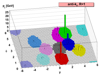
The result of the CMS Particle Flow algorithm is a list of particle candidates that account for all inner-tracker and muon tracks and all above-threshold energy deposits in the calorimeters. These particles are formed into jets using a “clustering algorithm”. The most common algorithm used by CMS is the “anti-kt” algorithm, which is abbreviated “AK”. It iterates over particle pairs and finds the two (i and j) that are the closest in some distance measure and determines whether to combine them:

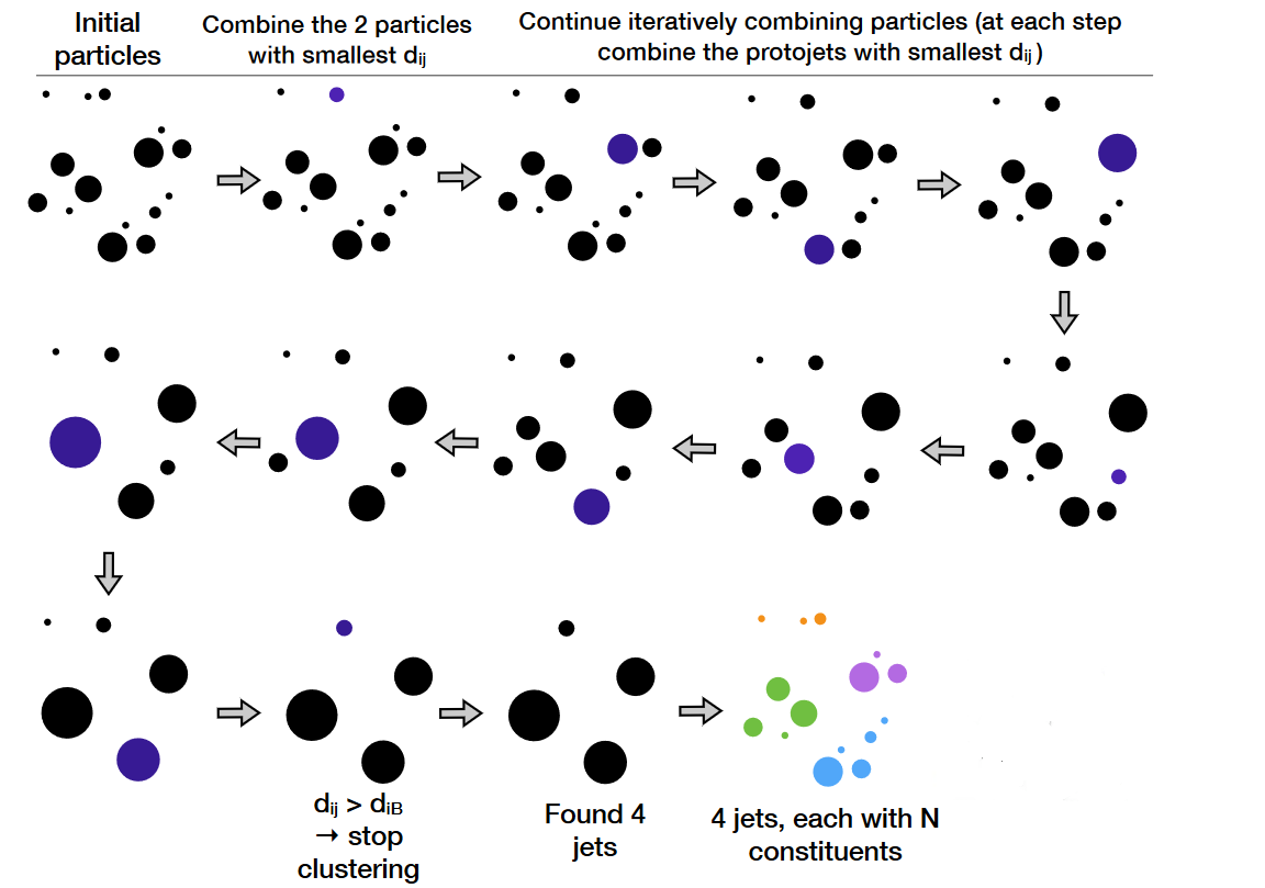
The momentum power (-2) used by the anti-kt algorithm means that higher-momentum particles are clustered first. This leads to jets with a round shape that tend to be centered on the hardest particle. In CMS software this clustering is implemented using the FastJet package.

Pileup

Inevitably, the list of particle flow candidates contains particles that did not originate from the primary interaction point. CMS experiences multiple simultaneous collisions, called “pileup”, during each “bunch crossing” of the LHC, so particles from multiple collisions coexist in the detector. There are various methods to remove their contributions from jets:

• Charged hadron subtraction CHS: all charged hadron candidates are associated with a track. If the track is not associated with the primary vertex, that charged hadron can be removed from the list. CHS is limited to the region of the detector covered by the inner tracker. The pileup contribution to neutral hadrons has to be removed mathematically – more in episode 3!
• PileUp Per Particle Identification (PUPPI, available in Run 2): CHS is applied, and then all remaining particles are weighted based on their likelihood of arising from pileup. This method is more stable and performant in high pileup scenarios such as the upcoming HL-LHC era.

Accessing jets in CMS software

Jets software classes have the same basic 4-vector methods as the objects discussed in the previous lesson. Beginning with the 2015 MiniAOD data files, the principle way to interact with jets in the OpenData files is via the pat::Jet class. PAT stands for “Physics Analysis Toolkit”, which is a framework for applying and accessing many common analysis-level algorithms that are used in CMS. The POET features JetAnalyzer.cc to demonstrate working with standard “small-radius” jets and FatjetAnalyzer.cc to demonstrate working with large-radius jets used in analyses of boosted SM particle decays.

In JetAnalyzer.cc

for (const pat::Jet &jet : *jets){ 

  ...
  jet_e.push_back(uncorrJet.energy());	// later we'll discuss "uncorr" and "smeared" and such!
  jet_pt.push_back(uncorrJet.pt());
  jet_eta.push_back(uncorrJet.eta());
  jet_phi.push_back(uncorrJet.phi());
  jet_ch.push_back(uncorrJet.charge());
  jet_mass.push_back(uncorrJet.mass());
  ...
  jet_corrpx.push_back(smearedjet.px());
  jet_corrpy.push_back(smearedjet.py());
  jet_corrpz.push_back(smearedjet.pz());  
  ...

}

Particle-flow jets are not immune to noise in the detector, and jets used in analyses should be filtered to remove noise jets. CMS has defined a Jet ID with criteria for good jets:

The PFlow jets are required to have charged hadron fraction CHF > 0.0 if within tracking fiducial region of |eta| < 2.4, neutral hadron fraction NHF < 1.0, charged electromagnetic (electron) fraction CEF < 1.0, and neutral electromagnetic (photon) fraction NEF < 1.0. These requirements remove fake jets arising from spurious energy depositions in a single sub-detector.

These criteria demonstrate how particle-flow jets combine information across subdetectors. Jets will typically have energy from electrons and photons, but those fractions of the total energy should be less than one. Similarly, jets should have some energy from charged hadrons if they overlap the inner tracker, and all the energy should not come from neutral hadrons. A mixture of energy sources is expected for genuine jets. All of these energy fractions (and more) can be accessed from the jet objects – but now with 2015 data, we can apply the noise ID filter for you!

In poet_cfg.py:

#----- Apply the noise jet ID filter -----#
process.looseAK4Jets = cms.EDFilter("PFJetIDSelectionFunctorFilter",
                                    filterParams = pfJetIDSelector.clone(),
                                    src = cms.InputTag("slimmedJets"))
process.looseAK8Jets = cms.EDFilter("PFJetIDSelectionFunctorFilter",
                                    filterParams = pfJetIDSelector.clone(),
                                    src = cms.InputTag("slimmedJetsAK8"))

MET

Missing transverse momentum is the negative vector sum of the transverse momenta of all particle flow candidates in an event. The magnitude of the missing transverse momentum vector is called missing transverse energy and referred to with the acronym “MET”. Since energy corrections are made to the particle flow jets, those corrections are propagated to MET by adding back the momentum vectors of the original jets and then subtracting the momentum vectors of the corrected jets. This correction is called “Type 1” and is standard for all CMS analyses. The POET has been configured to compute and apply the Type-1 correction for you automatically, starting from raw MET and using the set of fully corrected small-radius jets, as shown below.

In \poet_cfg.py:

#----- Evaluate the Type-1 correction -----#

process.Type1CorrForNewJEC = patPFMetT1T2Corr.clone(
        isMC = cms.bool(isMC),
        src = cms.InputTag("slimmedJetsNewJEC"),
        )
process.slimmedMETsNewJEC = cms.EDProducer('CorrectedPATMETProducer',
        src = cms.InputTag('uncorrectedPatMet'),
        srcCorrections = cms.VInputTag(cms.InputTag('Type1CorrForNewJEC', 'type1'))
        )

In MetAnalyzer.cc we open the particle flow MET module and extract the magnitude and angle of the MET, the sum of all energy in the detector, and variables related to the “significance” of the MET. Note that MET quantities have a single value for the entire event, unlike the objects studied previously. The raw MET values are also available for comparison.

Handle<pat::METCollection> mets;
iEvent.getByToken(metToken_, mets);

const pat::MET &met = mets->front();

met_e = met.sumEt();
met_pt = met.pt();
met_px = met.px();
met_py = met.py();
met_phi = met.phi();
met_significance = met.significance();
}

MET significance can be a useful tool: it describes the likelihood that the MET arose from noise or mismeasurement in the detector as opposed to a neutrino or similar non-interacting particle. The four-vectors of the other physics objects along with their uncertainties are required to compute the significance of the MET signature. MET that is directed nearly (anti)colinnear with a physics object is likely to arise from mismeasurement and should not have a large significance.

Key Points

• Jets are spatially-grouped collections of particles that traversed the CMS detector

• Particles from additional proton-proton collisions (pileup) must be removed from jets

• Missing transverse energy is the negative vector sum of particle candidates

• Many of the class methods discussed for other objects can be used for jets

Jet substructure

Overview

Teaching: 10 min
Exercises: 25 min

Questions

• Which jet substructure observables are available in CMS MiniAOD?

• How are W boson jets identified using fat jets?

• How are top quark jets identified using fat jets?

Objectives

• Understand the groomed mass and jet substructure variables typically used in CMS analyses

• Study W boson and top quark identification

Run POET (…maybe…)

If you have not already, run POET using the entire top quark pair test file. In python/poet_cfg.py set the number of events to process to -1:

#---- Select the maximum number of events to process (if -1, run over all events)
process.maxEvents = cms.untracked.PSet( input = cms.untracked.int32(-1) )

#---- Define the test source files to be read using the xrootd protocol (root://), or local files (file:)
process.source = cms.Source("PoolSource", fileNames = cms.untracked.vstring(
        'root://eospublic.cern.ch//eos/opendata/cms/mc/RunIIFall15MiniAODv2/TT_Mtt-1000toInf_TuneCUETP8M1_13TeV-powheg-pythia8/MINIAODSIM/PU25nsData2015v1_76X_mcRun2_asymptotic_v12_ext1-v1/80000/000D040B-4ED6-E511-91B6-002481CFC92C.root',
        )
)

And run POET using cmsRun python/poet_cfg.py.

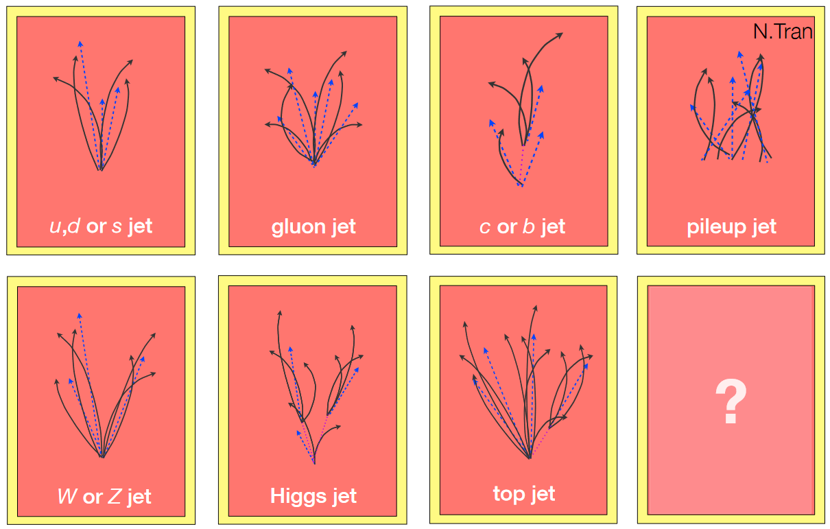
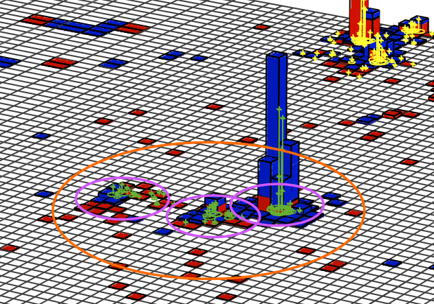
Jets can originate from many different types of particles. The figure below gives an example of how different “parent particles” can influence the internal structure of a jet. Observables related to the mass and internal structure of a jet can help us design algorithms to distinguish between sources. The most common type of algorithm identifies b quark jets from light quark or gluon jets. The POET contains all the tools you need to evaluate the default CMS b tagging discriminants on small-radius jets. See the next episode for more information. In this lesson we will focus on tools to identify hadronic decays of Lorentz-boosed massive SM particles within large-radius jets.

Jet mass and grooming

The mass of a jet is evaluated by summing the energy-momentum four-vectors of all the particle flow candidates that make up the jet and computing the mass of the resulting object. This mass calculation is distorted by the low-momentum and wide-angle gluon radiation emerging from the initial hadrons that formed the jet. For example, the masses of light quark or gluon jets are measured to be much larger than the actual masses of these particles – typically 10–50 GeV with a smooth continuum to higher values. Grooming procedures can help reduce the impact of this radiation and bring the jet mass closer to the true values of the parent particles. Grooming algorithms typically cluster the jet’s consitituents into “subjets”, like those represented by the small circles in the figure below. The relationships between different subjets can then be tested to decide which to keep.

Four groomed masses are available for large-radius (“fat”) jets in 2015 MiniAOD:

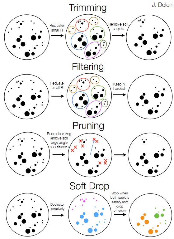
• Trimmed mass: jets are reclustered using a small distance parameter, and any “subjets” that have too small a fraction of the original jet momentum are discarded.
• Filtered mass: jets are reclustered using a small distance parameter, and a certain number of subjets are kept.
• Pruned mass (default for identifying W/Z/H boson jets): jets are reclustered, and at each step subjets that are too soft or at large angles are discarded.
• Soft drop mass (default for identifying t quark jets): jets are recursively de-clustered, and at each step jets that are too soft or at large angles are discarded.

In FatjetAnalyzer.cc the groomed masses are accessed via the “userFloat” method available in all PAT classes. This implies that a value has been calculated elsewhere and the result stored manually inside the PAT object. In the case of jet masses, it is important to note that userFloat values are not automatically corrected when “jet energy corrections” are applied. These corrections are covered in the last segment of this lesson – in POET specific levels of correction are applied to the groomed masses.

fatjet_prunedmass.push_back(corrL2L3*(double)smearedFatjet.userFloat("ak8PFJetsCHSPrunedMass"));
fatjet_softdropmass.push_back(corrL2L3*(double)smearedFatjet.userFloat("ak8PFJetsCHSSoftDropMass"));

Exercise: boosted particle momentum ranges

Study the connection between jet mass and jet momentum – what minimum transverse momentum is required for W boson and top quark jets to be found within a large-radius jet?

Begin by opening the myoutput.root file you processed at the beginning of this segment. Use ROOT’s capability to draw two-dimensional histograms to compare various jet masses against the jet’s transverse momentum:

$ root -l myoutput.root
[1] _file0->cd("myfatjets");
[2] Events->Draw("fatjet_<SOME MASS VARIABLE>:fatjet_corrpt","","colz"); // colz makes a heatmap

Solution

This plot shows the relationship between momentum, mass, and jet radius. As the momentum increases, jets of larger mass become contained within the fat jet. While W bosons can be observed from 200 GeV, top quarks require a higher momentum threshold.

Jet substructure

The internal structure of a jet can be probed using many observables: N-subjettiness, energy correlation functions, and others. In CMS, N-subjettiness is the default jet substructure variable for identifying boosted particle decays.

The “tau” variables of N-subjettiness, defined below, are jet shape variables whose value approaches 0 for jets having N or fewer subjets:

If the value approaches zero it indicates that the consitituents all lie near one of the previously identified subjet axes. For a top quark jet with 3 subjets, we would expect small tau values for N = 3, 4, 5, 6, etc, but larger values for N = 1 or 2.

Ratios of tau values provide the best discrimination for jets with a specific number of subjets. For two-prong jets like W, Z, or H boson decays, we study the ratio tau_2 / tau_1. For three-prong jets we study tau_3 / tau_2.

In FatjetAnalyzer.cc, the N-subjettiness values are also accessed from userFloats:

fatjet_tau1.push_back((double)smearedFatjet.userFloat("NjettinessAK8:tau1"));
fatjet_tau2.push_back((double)smearedFatjet.userFloat("NjettinessAK8:tau2"));
fatjet_tau3.push_back((double)smearedFatjet.userFloat("NjettinessAK8:tau3"));

For top quark or H boson decays, applying b tagging algorithms to the subjets of the large-radius jets gives another valuable substructure observable. The Combined Secondary Vertex v2 discriminant, described in detail in the next episode, has been stored for the two subjets obtained from the soft drop algorithm in each large-radius jet. For simulation, we also store the generator-level flavor information for the subjet.

auto const & sdSubjets = smearedFatjet.subjets("SoftDrop");
int nSDSubJets = sdSubjets.size();
if(nSDSubJets > 0){
    pat::Jet subjet1 = sdSubjets.at(0);
    fatjet_subjet1btag.push_back(subjet1.bDiscriminator("pfCombinedInclusiveSecondaryVertexV2BJetTags"));
    fatjet_subjet1hflav.push_back(subjet1.hadronFlavour());
}else{
    fatjet_subjet1btag.push_back(-999);
    fatjet_subjet1hflav.push_back(-999);
}
// then the same for the 2nd subjet

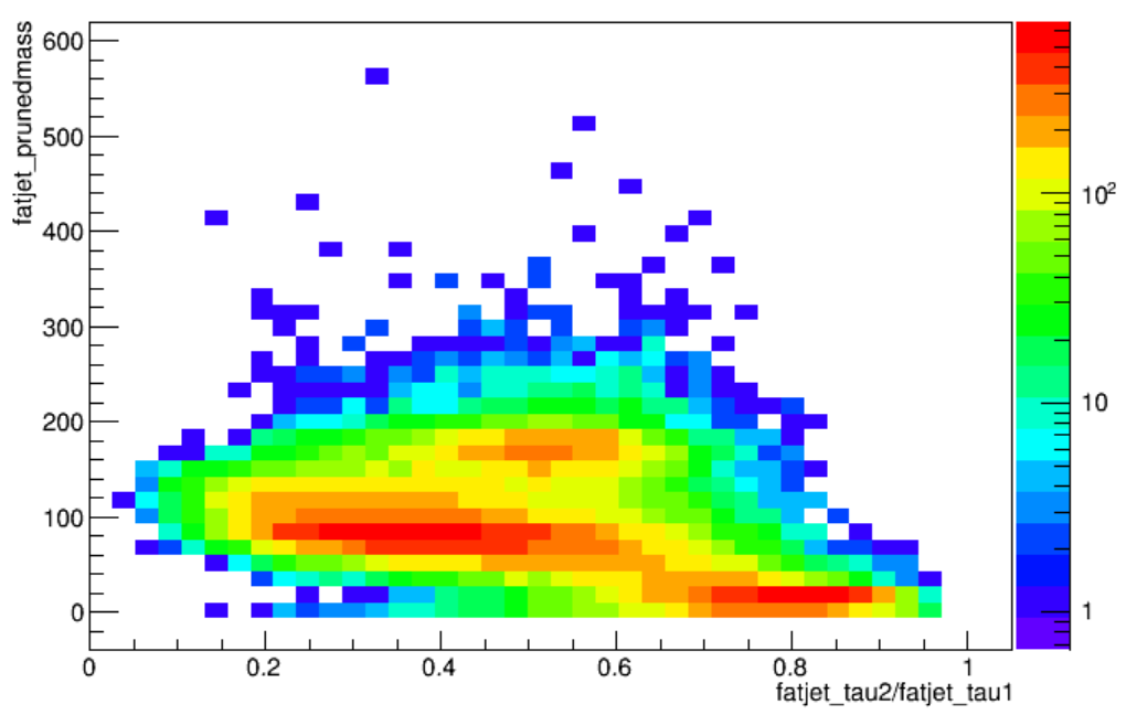
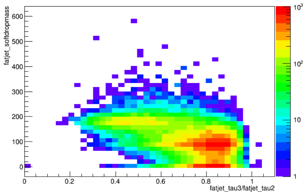
Exercise: mass and N-subjettiness correlations

Study the correlation between groomed jet mass and N-subjettiness ratios. Make 2D plots of either pruned jet mass versus tau_2/tau_1, or softdrop jet mass versus tau_3/tau_2. Where do the various parent particles of the jets pool? What requirements would effectively select W bosons or top quarks? Tip: use the same type of ROOT Draw command as in the previous exercise.

Solution

The structure in the tau_2/tau_1 plot is very unique: W bosons pool at lower values of tau_2/tau_1, while top quarks (with more than 2 subjets) and light quarks (with only 1 subjet) pool at medium and higher values. In the tau_3/tau_2 plot, top quark jets have low values while both W boson and light quark jets are gathered near 1. The correlations in these plots lead directly to the “tagging” criteria introduced in the next section.

W and top tagging

The CMS jet algorithms group studied the efficiency of identifying known W boson jets using almost 30 different combinations of groomed mass and jet substructure variables. The optimal combination for 2015 data was pruned mass + tau_2/tau_1 for large-radius jets using the CHS pileup mitigation technique. For “PUPPI” jets, developed for Run 2, the softdrop mass is used instead. The use of PUPPI jets became the default for CMS analyses beginning only in 2016, so currently this option is not implemented in the POET.

Selection criteria for W boson and top quark jets in 2015 data analyses are described in this Physics Analysis Summary, including the calculations of corrections factors for simulation.

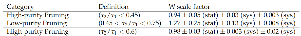
W boson selections

A W jet has pruned mass between 65 – 105 GeV and tau_2/tau_1 less than a chosen upper bound. The supported working points and their correction factors are shown in this table:

For top quarks, the soft drop mass is used regardless of pileup mitigation technique for the jets. In this case, tau_3/tau_2 becomes the most useful substructure variable, followed by b quark tagging applied on the individual subjets of the large-radius jet.

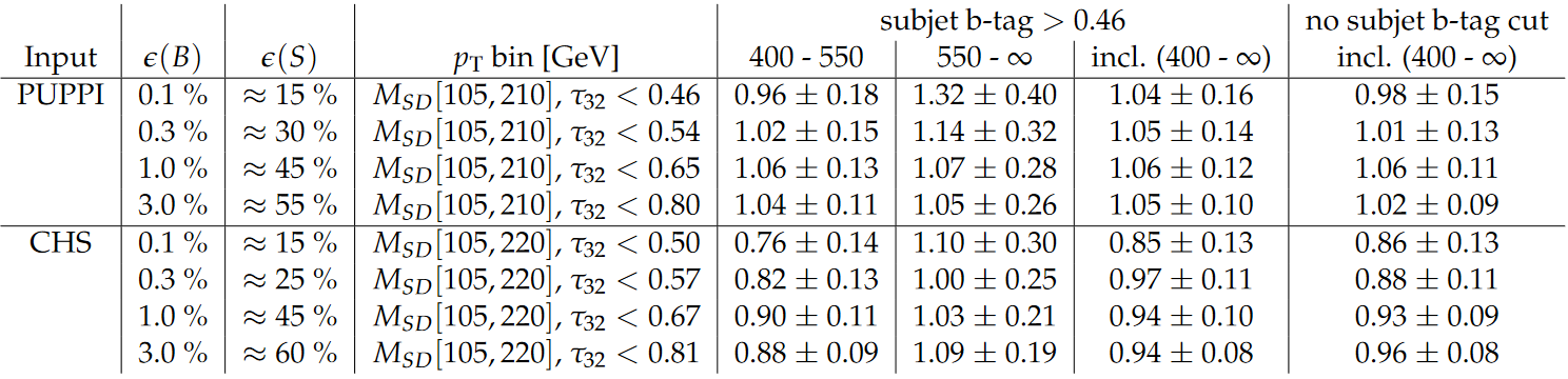
Top quark selections

A top quark jet has soft drop mass between 105 – 220 GeV, tau_3/tau_2 less than a chosen upper bound, and possibly a requirement on a subjet b quark tag. The supported working points, their efficiencies, and correction factors are shown in this table:

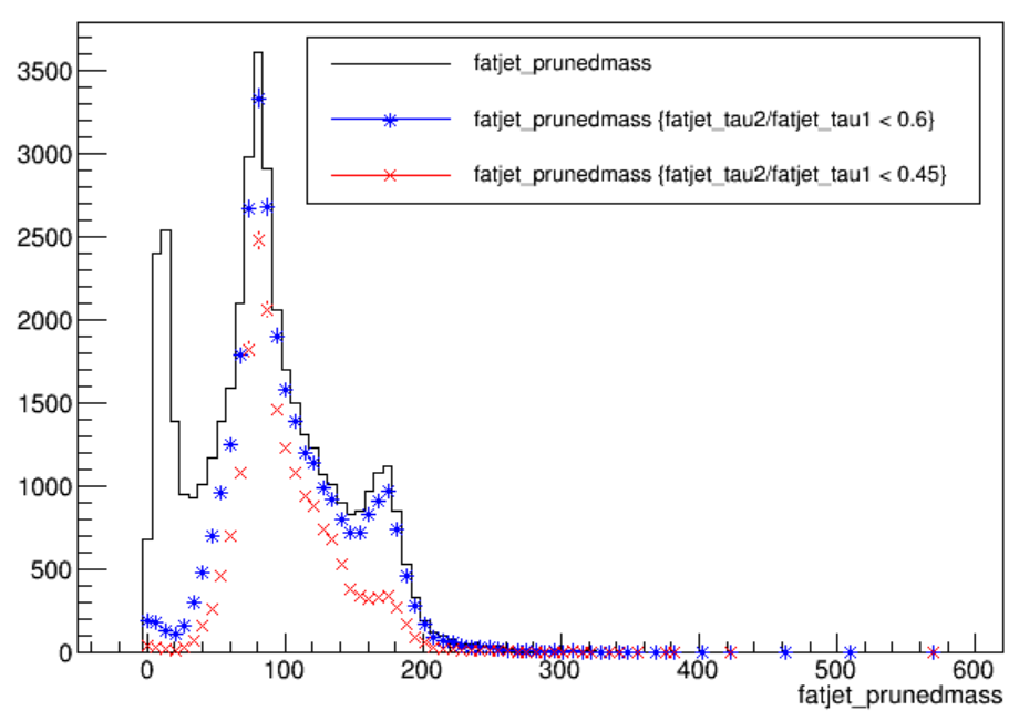
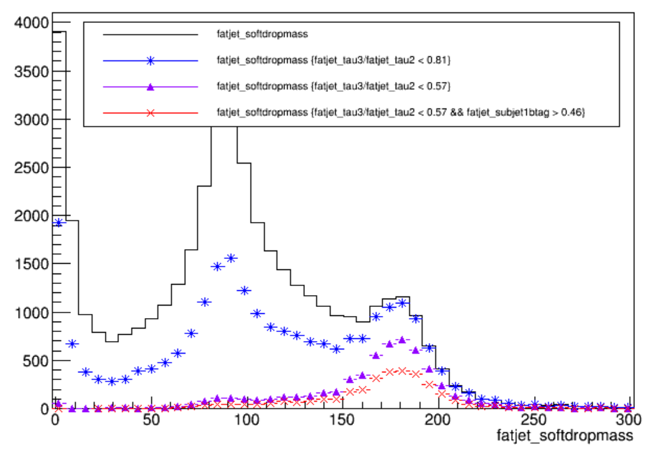
Exercise: explore jet tagging criteria

Study the connection between groomed mass, n-subjettiness ratios, and subjet b-tagging. From the top quark events in myoutput.root, can you see either a W boson or top quark mass peak become visible in the fatjet_prunedmass or fatjet_softdropmass distribution as you apply the various substructure criteria?

Recall: Events->Draw("fatjet_X","fatjet_Y > VALUE") will draw the branch fatjet_X for all events in which fatjet_Y > VALUE. Adding a third parameter to the Draw command that says “same” will place a new histogram on top of any existing histograms.

Criteria you could test include:

• fatjet_tau2/fatjet_tau1 < 0.6
• fatjet_tau2/fatjet_tau1 < 0.45
• fatjet_corrpt > 500
• fatjet_tau3/fatjet_tau2 < 0.81
• fatjet_tau3/fatjet_tau2 < 0.57
• fatjet_subjet1btag > .046

Solution

Both the W boson jets and the top quark jets can be isolated from the other jet types quite effectively with the N-subjettiness criteria!

Key Points

• Grooming algorithms remove soft and wide angle radiation to bring a jet’s mass closer to that of the parent particle.

• Substructure algorithms provide information about the number of high-momentum subjets or whether heavy flavor hadrons existed inside the jet.

• The standard variables needed to tag W, Z, H boson or top quark jets in 2015 data are included in the POET.

Extra reading: Heavy flavor tagging

Overview

Teaching: 0 (15 min) min
Exercises: min

Questions

• How are b hadrons identified in CMS

Objectives

• Understand the basics of heavy flavor tagging

• Learn to access tagging information in MiniAOD files

Jet reconstruction and identification is an important part of the analyses at the LHC. A jet may contain the hadronization products of any quark or gluon, or possibly the decay products of more massive particles such as W or Higgs bosons. Several “b tagging” algorithms exist to identify jets from the hadronization of b quarks, which have unique properties that distinguish them from light quark or gluon jets.

B Tagging Algorithms

Tagging algorithms first connect the jets with good quality tracks that are either associated with one of the jet’s particle flow candidates or within a nearby cone. Both tracks and “secondary vertices” (track vertices from the decays of b hadrons) can be used in track-based, vertex-based, or “combined” tagging algorithms. The specific details depend upon the algorithm use. However, they all exploit properties of b hadrons such as:

• long lifetime,
• large mass,
• high track multiplicity,
• large semileptonic branching fraction,
• hard fragmentation fuction.

Tagging algorithms are Algorithms that are used for b-tagging:

• Track Counting: identifies a b jet if it contains at least N tracks with significantly non-zero impact parameters.
• Jet Probability: combines information from all selected tracks in the jet and uses probability density functions to assign a probability to each track
• Soft Muon and Soft Electron: identifies b jets by searching for a lepton from a semi-leptonic b decay.
• Simple Secondary Vertex: reconstructs the b decay vertex and calculates a discriminator using related kinematic variables.
• Combined Secondary Vertex: exploits all known kinematic variables of the jets, information about track impact parameter significance and the secondary vertices to distinguish b jets. This tagger became the default CMS algorithm.

These algorithms produce a single, real number (often the output of an MVA) called a b tagging “discriminator” for each jet. The more positive the discriminator value, the more likely it is that this jet contained b hadrons.

Accessing tagging information

In JetAnalyzer.cc we access the information from the Combined Secondary Vertex V2 (CSV) b tagging algorithm and associate discriminator values with the jets. During the creation of pat::Jet objects, this information is merged into the jets so that the discriminators can be accessed with a dedicated member function (similar merging is done for other useful associations like generated jets and jet flavor in simulation!).

jet_btag.push_back(itjet->bDiscriminator("combinedSecondaryVertexBJetTags"));

We can investigate at the b tag information in a dataset using ROOT.

$ root -l myoutput.root // you produced this earlier in hands-on exercise #2
[0] _file0->cd("myjets");
[1] Events->Draw("jet_btag");

The discriminator values for jets with kinematics in the correct range for this algorithm lie between 0 and 1. Other jets that do not have a valid discriminator value pick up values of -1, -9, or -999.

Working points

A jet is considered “b tagged” if the discriminator value exceeds some threshold. Different thresholds will have different efficiencies for identifying true b quark jets and for mis-tagging light quark jets. As we saw for muons and other objects, a “loose” working point will allow the highest mis-tagging rate, while a “tight” working point will sacrifice some correct-tag efficiency to reduce mis-tagging. The CSVv2 algorithm has working points defined based on mis-tagging rate (read more):

• Loose = ~10% mis-tagging = discriminator > 0.460
• Medium = ~1% mis-tagging = discriminator > 0.800
• Tight = ~0.1% mis-tagging = discriminator > 0.935

The figure below shows the relationship between b jet efficiency and misidentification rate in several b tagging algorithms, including CSVv2 (read more).

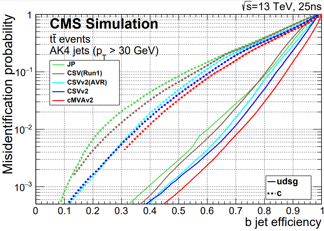
Applying scale factors

Scale factors to increase or decrease the number of b-tagged jets in simulation can be applied in a number of ways, but typically involve weighting simulation events based on the efficiencies and scale factors relevant to each jet in the event. Scale factors for the CSVv2 algorithm are described in the reference linked above, and have been implemented in the POET. Details and usage references from Run 1 can be found at these references:

• Explanation
• Data file for the CSV algoritm
• Examples of application methods

In POET, the scale factor functions for the CSVv2 Medium working point have been implemented in JetAnalyzer.cc. The scale factor is a single numerical value calculated from a function of the corrected jet momentum:

double JetAnalyzer::getBorCtagSF(double pt, double eta){
  if(pt > 670) pt = 670;
  if(fabs(eta) > 2.4 or pt < 30.) return 1.0;

  return 0.934588*((1.+(0.00678184*pt))/(1.+(0.00627144*pt)));
}

The most commonly used method to apply scale factors is Method 1a, and it has been implemented in POET. This is an event weight method of applying a correction, so the final result is an event weight to be stored for later in the analysis, along with extra event weights to describe the uncertainty.

The method relies on 4 pieces of information for each jet in simulation:

• Tagging status: does this jet pass the discriminator threshold for a given working point?
• Flavor (b, c, light): accessed using a pat::Jet member function called partonFlavour().
• Efficiency: accessed from the lookup functions based on the jet’s momentum.
• Scale factor: accessed from the helper functions based on the jet’s momentum.

Each jet then contributes to the event weight based on these four features. For example, jets that pass the discriminator threshold and are b quark jets contribute the following factor to variables called MC, which appears as P(MC) in the reference TWiki, and btagWeight, which appears as P(DATA) in the reference TWiki.

hadronFlavour = smearedjet.hadronFlavour();
corrpt = jet_corrpt.at(numjet);       
 
if (jet_btag.at(numjet)> 0.800){ // MEDIUM working point
    if(abs(hadronFlavour) == 5){
        eff = getBtagEfficiency(corrpt);
        SF = getBorCtagSF(corrpt, jet_eta.at(numjet));
        SFu = SF + uncertaintyForBTagSF(corrpt, jet_eta.at(numjet));
        SFd = SF - uncertaintyForBTagSF(corrpt, jet_eta.at(numjet));
    }
    // ... repeat for c and light quark jets...

    MC *= eff;
    btagWeight *= SF * eff;
    btagWeightUp *= SFu * eff;
    btagWeightDn *= SFd * eff;
}
//...similar for non-tagged jets...

After the jet loop, the reference TWiki defines the weight as P(DATA)/P(MC):

btagWeight = (btagWeight/MC);
btagWeightUp = (btagWeightUp/MC);
btagWeightDn = (btagWeightDn/MC);

The weight and its uncertainties are all stored in the tree for use later in filling histograms.

Key Points

• Tagging algorithms separate heavy flavor jets from jets produced by the hadronization of light quarks and gluons

• Tagging algorithms produce a disriminator value for each jet that represents the likelihood that the jet came from a b hadron

• Each tagging algorithm has recommended ‘working points’ (discriminator values) based on a misidentification probability for light-flavor jets

Extra reading: Jet corrections

Overview

Teaching: 0 (15 min) min
Exercises: 0 (30 min) min

Questions

• How are data/simulation differences dealt with for jet energy?

• How do uncorrected and corrected jet momenta compare?

• How large is the JEC uncertainty in different regions?

• How large is the JER uncertainty in different regions?

Objectives

• Learn about typical differences in jet energy scale and resolution between data and simulation

• Learn how JEC and JER corrections can be applied to OpenData jets

• Access uncertainties in both JEC and JER

• Explore the JEC and JER uncertainties using histograms

• Practice basic plotting with ROOT

Unsurprisingly, the CMS detector does not measure jet energies perfectly, nor do simulation and data agree perfectly! The measured energy of jet must be corrected so that it can be related to the true energy of its parent particle. These corrections account for several effects and are factorized so that each effect can be studied independently. All of the corrections in this section are described in “Jet Energy Scale and Resolution” papers by CMS:

• 2011, 7 TeV
• 2017, 8 TeV

Correction levels

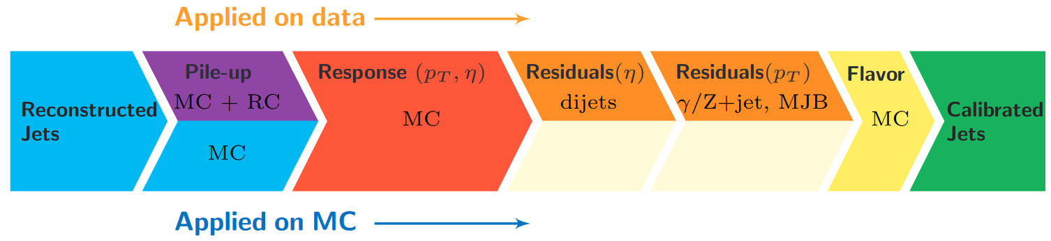
Particles from additional interactions in nearby bunch crossings of the LHC contribute energy in the calorimeters that must somehow be distinguished from the energy deposits of the main interaction. Extra energy in a jet’s cone can make its measured momentum larger than the momentum of the parent particle. The first layer (“L1”) of jet energy corrections accounts for pileup by subtracting the average transverse momentum contribution of the pileup interactions to the jet’s cone area. This average pileup contribution varies by pseudorapidity and, of course, by the number of interactions in the event.

The second and third layers of corrections (“L2L3”) correct the measured momentum to the true momentum as functions of momentum and pseudorapidity, bringing the reconstructed jet in line with the generated jet. These corrections are derived using momentum balancing and missing energy techniques in dijet and Z boson events. One well-measured object (ex: a jet near the center of the detector, a Z boson reconstructed from leptons) is balanced against a jet for which corrections are derived.

All of these corrections are applied to both data and simulation. Data events are then given “residual” corrections to bring data into line with the corrected simulation. A final set of flavor-based corrections are used in certain analyses that are especially sensitive to flavor effects. The figure below shows the result of the L1+L2+L3 corrections on the jet response.

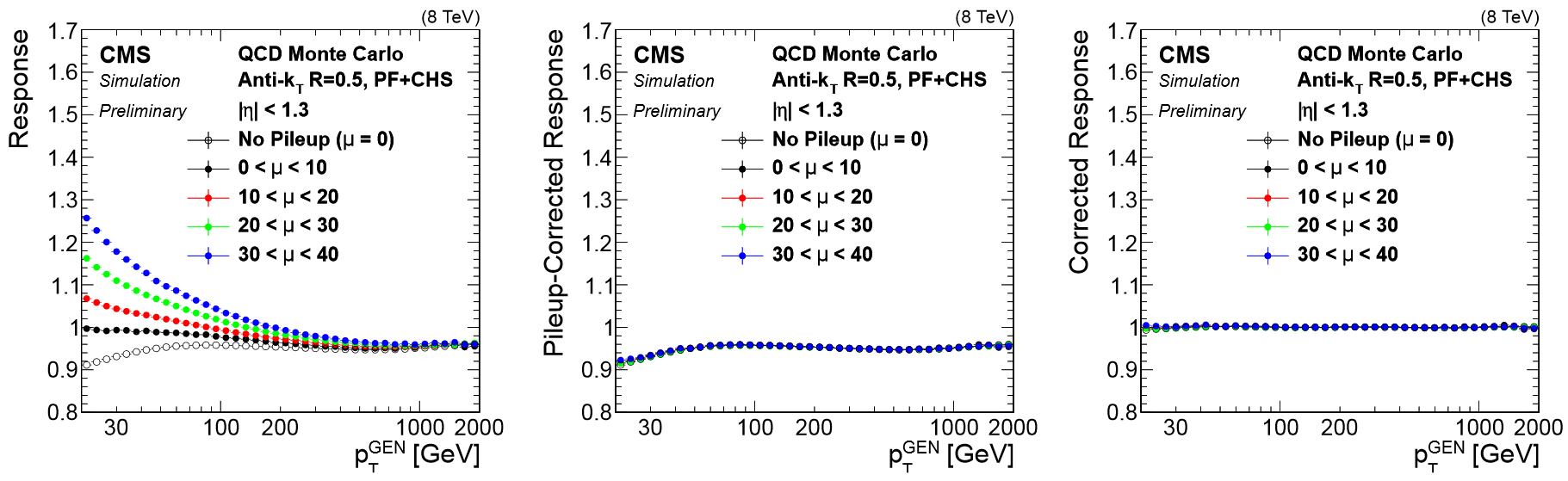
Jet Energy Resolution

Jet Energy Resolution (JER) corrections are applied after JEC on strictly MC simulations. Unlike JEC, which adjusts the mean of the momentun response distribution, JER adjusts the width of the distribution. The ratio of reconstructed transverse momentum to true (generated) transverse momentum forms a Gaussian distributions – the width of this Gaussian is the JER. In data, where no “true” pT is available, the JER is measured using photon/Z + jet events where the jet recoils against the photon or Z boson, both of which can be measured quite precisely in the CMS detector. The JER is typically smaller in simulation than in data, leading to scale factors that are larger than 1. These scale factors, along with their uncertainties, are accessible in POET in the jet analyzers. They are applied using two methods:

• Adjusting the ratio of reconstructed to generated momentum using the scale factor (if a well-matched generated jet is found),
• Randomly smearing the momentum using a Gaussian distribution based on the resolution and scale factor (if no generated jet is found).

Applying JEC and JER

The jet energy corrections and Type-1 MET corrections are applied to both small-radius and large-radius jets when you run POET. The segments shown below create two collections of jets called slimmedJetsNewNEC and slimmedJetsAK8NewJEC. These collections will then be opened in the jet analyzers. In poet_cfg.py:

#----- Apply the final jet energy corrections for 2015 -----#
process.patJetCorrFactorsReapplyJEC = updatedPatJetCorrFactors.clone(src = cms.InputTag("looseAK4Jets"))
if isData: process.patJetCorrFactorsReapplyJEC.levels.append('L2L3Residual')
process.slimmedJetsNewJEC = updatedPatJets.clone(
    jetSource = cms.InputTag("looseAK4Jets"),
    jetCorrFactorsSource = cms.VInputTag(cms.InputTag("patJetCorrFactorsReapplyJEC")),
)
process.patJetCorrFactorsReapplyJECAK8 = updatedPatJetCorrFactors.clone(
        src = cms.InputTag("looseAK8Jets"),
        levels = ['L1FastJet', 'L2Relative', 'L3Absolute'],
        payload = 'AK8PFchs'
        )
if isData: process.patJetCorrFactorsReapplyJECAK8.levels.append('L2L3Residual')
process.slimmedJetsAK8NewJEC = updatedPatJets.clone(
    jetSource = cms.InputTag("looseAK8Jets"),
    jetCorrFactorsSource = cms.VInputTag(cms.InputTag("patJetCorrFactorsReapplyJECAK8")),
)

In the jet analyzers, the “default” jets now have the jet energy corrections applied! But we can still access the “uncorrected jet” from any pat::Jet object:

for (const pat::Jet &jet : *jets){
  pat::Jet uncorrJet = jet.correctedJet(0);

  // jet is the corrected jet and uncorrJet is the raw jet
}

The JER corrections must be accessed from a text file and applied on top of the corrected jets. Helper classes called JetResolution and JetResolutionScaleFactor provide access to the scale factors and jet momentum resolutions stored in the text files.

In the constructor function JetAnalyzer::JetAnalyzer:

jerResName_(iConfig.getParameter<edm::FileInPath>("jerResName").fullPath()),; // JER Resolutions                               
sfName_(iConfig.getParameter<edm::FileInPath>("jerSFName").fullPath()), // JER Resolutions

resolution = JME::JetResolution(jetResName_);
resolution_sf = JME::JetResolutionScaleFactor(sfName_);

We can now use jer_->correction() to access the jet’s momentum resolution in simulation. In the code snippet below you can see “scaling” and “smearing” versions of applying the JER scale factors, depending on whether or not this pat::Jet had a matched generated jet. The random smearing application uses a reproducible seed for the random number generator based on the inherently random azimuthal angle of the jet.

Note: this code snippet is simplified by removing lines for handling uncertainties – that’s coming below!

for (const pat::Jet &jet : *jets){

    ptscale = 1;
    if(!isData) {

        JME::JetParameters JERparameters = { {JME::Binning::JetPt, corrpt}, {JME::Binning::JetEta, jet.eta()}, {JME::Binning::Rho, *(rhoHandle.product())} };
    	float res = resolution.getResolution(JERparameters); 
    	float sf = resolution_sf.getScaleFactor(JERparameters);
    	float sf_up = resolution_sf.getScaleFactor(JERparameters, Variation::UP);
    	float sf_down = resolution_sf.getScaleFactor(JERparameters, Variation::DOWN);

    	const reco::GenJet *genJet = jet.genJet();
    	bool smeared = false;
    	if(genJet){
    	    double deltaPt = fabs(genJet->pt() - corrpt);
   	    double deltaR = reco::deltaR(genJet->p4(),jet.p4());
   	    if ((deltaR < 0.2) && deltaPt <= 3*corrpt*res){
     	        ptscale = max(0.0, 1 + (sf - 1.0)*(corrpt - genJet->pt())/corrpt);
     	    	smeared = true;
   	    }
        } 
        if (!smeared) {
            TRandom3 JERrand;
   
	    JERrand.SetSeed(abs(static_cast<int>(jet.phi()*1e4)));
   	    ptscale = max(0.0, 1.0 + JERrand.Gaus(0, res)*sqrt(max(0.0, sf*sf - 1.0)));
        }
     }
     if( ptscale*corrpt <= min_pt) continue;

     pat::Jet smearedjet = jet;
     smearedjet.scaleEnergy(ptscale);
}

The final, definitive jet momentum is the raw momentum multiplied by both JEC and JER corrections! After computing ptscale, we store a variety of corrected and uncorrected kinematic variables for jets passing the momentum threshold.

Uncertainties

You will have noticed that nested among the JEC and JER code snippets given above were commands related to the uncertainty in these corrections. The JEC uncertainties have several sources, shown in the figure below. The L1 (pileup) uncertainty dominates at low momentum, while the L3 (absolute scale) uncertainty takes over for higher momentum jets. All corrections are quite precise for jets located near the center of the CMS barrel region, and the precision drops as pseudorapidity increases and different subdetectors lose coverage.

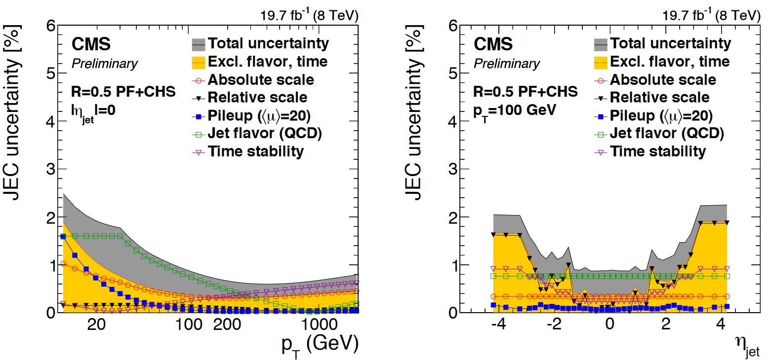
The JER uncertainty is evaluated by shifting the scale factors up and down according to the error bars shown in the scale factor figure above. These uncertainties arise from treatment of initial and final state radiation in the data measurement, differences in Monte Carlo tunes across generator platforms, and small non-Gaussian tail effects.

The JEC uncertainty text file is loaded as a JetCorrectionUncertainty object in the JetAnalyzer constructor:

jetJECUncName_(iConfig.getParameter<edm::FileInPath>("jetJECUncName").fullPath()), // JEC uncertainties

jecUnc_ = boost::shared_ptr<JetCorrectionUncertainty>( new JetCorrectionUncertainty(jecJECUncName_) );

This object provides a getUncertainty() function that takes in the jet’s momentum and pseudorapidity and returns an adjustment to the JEC correction factor:

for (const pat::Jet &jet : *jets){

    corrpt = jet.pt();
    corrUp = 1.0;
    corrDown = 1.0;

    if( fabs(jet.eta()) < 5) jecUnc_->setJetEta( jet.eta() );
    else jecUnc_->setJetEta( 4.99 );
    jecUnc_->setJetPt( corrpt );
    corrUp = (1 + fabs(jecUnc_->getUncertainty(1)));

    if( fabs(jet.eta()) < 5) jecUnc_->setJetEta( jet.eta() );
    else jecUnc_->setJetEta( 4.99 );
    jecUnc_->setJetPt( corrpt );
    corrDown = (1 - fabs(jecUnc_->getUncertainty(-1)));        

The JER uncertainty is evaluated by calculating a ptscale_up and ptscale_down correction, exactly as shown above for the ptscale correction, but using the shifted scale factors. The uncertainties in JEC and JER are kept separate from each other: when varying JEC, the JER correction is held constant, and vice versa. This results in 5 momentum branches: a central value and two sets of uncertainties:

jet_corrpt.push_back(smearedjet.pt());
jet_corrptUp.push_back(corrUp*smearedjet.pt());
jet_corrptDown.push_back(corrDown*smearedjet.pt());
jet_corrptSmearUp.push_back(ptscale_up*smearedjet.pt()/ptscale);
jet_corrptSmearDown.push_back(ptscale_down*smearedjet.pt()/ptscale);

Challenge activity (with solutions_

Open myoutput.root and investigate the range of momentum variation given by the JEC uncertainties by plotting:

• Corrected versus uncorrected jet momentum
• Corrected jet momentum with JEC up and down uncertainties
• Corrected jet momentum with JER up and down uncertainties

Questions:

Is the difference between the raw and corrected momentum larger or smaller than the uncertainty? Which uncertainty dominates?

Solution

The following plotting commands can be used to draw the four histograms needed to answer the first question:

$ root -l myoutput.root
[1] _file0->cd("myjets");
[2] Events->Draw("jet_pt");
[3] Events->Draw("jet_corrpt","","hist same");
[4] Events->Draw("jet_corrptUp","","hist same");
[5] Events->Draw("jet_corrptDown","","hist same");

We can see that the corrections are significant, far larger than the uncertainty itself. The first level of correction, for pileup removal, tends to reduce the momentum of the jet. The JER uncertainty can be drawn using similar commands:

This uncertainty is much smaller for the majority of jets! The JER correction is similar to the muon Rochester corrections in that it is most important for analyses requiring higher precision in jet agreement between data and simulation.

Repeat these plots with the additional requirement that the jets be “forward” (abs(jet_eta) > 3.0) How do the magnitudes of the uncertainties compare in this region?

Solution

This time we need to apply cuts to the jets as we draw:

$ root -l myoutput.root
[1] _file0->cd("myjets");
[2] Events->Draw("jet_pt","abs(jet_eta) > 3.0");
[3] Events->Draw("jet_corrpt","abs(jet_eta) > 3.0","hist same");
[4] Events->Draw("jet_corrptUp","abs(jet_eta) > 3.0","hist same");
[5] Events->Draw("jet_corrptDown","abs(jet_eta) > 3.0","hist same");

In the endcap region the uncertainty on the JER scale factor has become nearly 20%! So this uncertainty gains almost equal footing with JEC. Many CMS analyses restrict themselves to studying jets in the “central” region of the detector, defined loosely by the tracker acceptance region of abs(eta) < 2.4 precisely to avoid these larger JEC and JER uncertainties.

Key Points

• Jet energy corrections are factorized and account for many mismeasurement effects

• L1+L2+L3 should be applied to jets used for analyses, with residual corrections for data

• Jet energy resolution in simulation is typically too narrow and is smeared using scale factors

• Jet energy and resolution corrections are sources of systematic error and uncertainties should be evaluated

• In general, the jet corrections are significant and lower the momenta of the jets with standard LHC pileup conditions.

• For most jets, the JEC uncertainty dominates over the JER uncertainty.

• In the endcap region of the detector, the JER uncertainty in larger and matches the JEC uncertainty.