CMS Data Flow
Overview
Teaching: 15 min
Exercises: 0 minQuestions
What does CMS do to process raw data into AOD and NanoAOD files?
Objectives
Review the flow of CMS data processing
CMS data follows a complex processing path after making it through the trigger selections you learned about in a previous lesson. The primary datasets begin with raw data events that have passed one or more of a certain set of triggers. For this workshop our test case is Higgs -> tau tau, so we analyze events in the “TauPlusX” primary dataset. Other datasets are defined for muon, electron, jet, MET, b-tagging, charmonium, and other trigger sets.
Skimming
Performing physics analyses with the raw primary datasets would be impossible! The datasets go through a processing of skimming (or also slimming, thinning, etc) to reduce their size and increase their usability – both by reducing the number of events and compressing the event format by removing information that is no longer needed. Data is processed through the following steps:
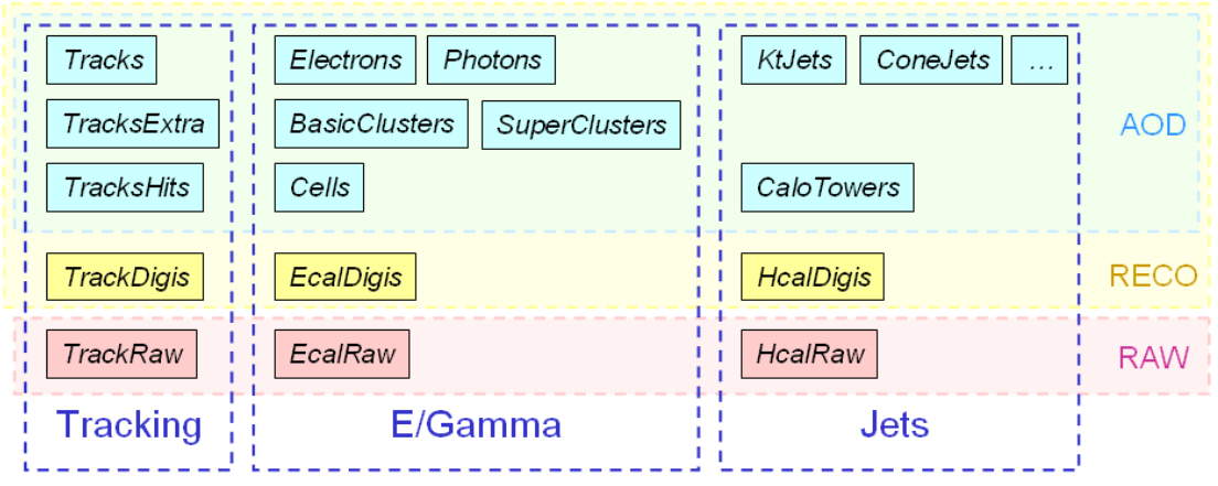
- RAW -> RECO: first reconstruction. Detector-level information is passed through reconstruction algorithms. Tracking, vertexing, and particle flow are performed in this step and basic physics object collections are created. Very CPU-intensive!
- RECO -> AOD: reduction to objects (Analysis Object Data). Only some hits and other detector-level info is kept, prioritizing physics object collections and some supporting information from RECO. In Run 1 this size file was suitable for analyzers.
- AOD -> MiniAOD: slimming of objects. AOD-level objects are passed through more selection and standard algorithms are run (such as JEC) so that information can be discarded. The MiniAOD format is based on CMS’s “Physics Analysis Toolkit” (PAT) object classes, which were originally developed for analysis-specific skims of AOD files.
- MiniAOD -> NanoAOD: further slimming of objects and flattening of the tree format. NanoAOD is currently the most compact CMS analysis format that contains only information about high-level objects in a “flat” ROOT tree format. NanoAOD is expected to have enough information for about 50% of CMS analyses.
The figure below shows example for tracking, ECAL, and HCAL-based objects.
Storage & processing
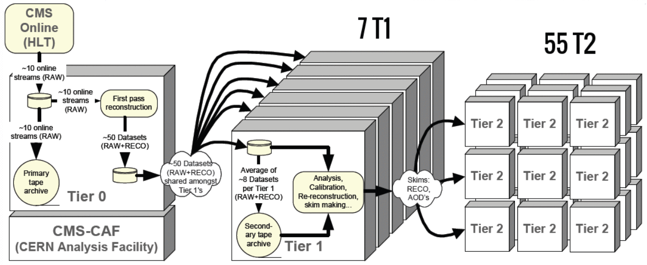
As the data is being skimmed it is also moving around the world. All RAW data is stored on tape in two copies, and the the RECO and AOD files are stored at various “tier 1” and “tier 2” computing centers around the world. The major Tier 1 center for the USA is at Fermilab. Several “tier 3” computing centers exist at universities and labs to store user-derived data for physics analyses.
More information about the CMS data flow can be found in the public workbook.
Key Points
Compression and selections happen at most levels of CMS data processing
Preselection in OpenData NanoAOD
Overview
Teaching: 10 min
Exercises: 0 minQuestions
What selections have been made when producing NanoAOD files?
Objectives
Summarize selections on objects made during NanoAOD production
Let’s review the selections made in the production of the NanoAOD files for this exercise. Data coming off the detector is already skimmed by the hardware triggers, and some further skimming is done when creating object collections, but we will concentrate on the final step of producing an “end user” ROOT file.
Triggers
The trigger list is slimmed to only 3 paths for these NanoAOD samples! In order to perform other analyses that required other triggers, new NanoAOD would need to be produced. This is an example of “analysis-specific” code verses more general CMS NanoAOD that contains the pass information for many more trigger paths. In the trigger manipulation lesson you learned methods to find trigger paths that could be added to the “interestingTriggers” list below for other physics analyses.
const static std::vector<std::string> interestingTriggers = {
    "HLT_IsoMu24_eta2p1",
    "HLT_IsoMu24",
    "HLT_IsoMu17_eta2p1_LooseIsoPFTau20",
};

// Trigger results
Handle<TriggerResults> trigger;
iEvent.getByLabel(InputTag("TriggerResults", "", "HLT"), trigger);
auto psetRegistry = edm::pset::Registry::instance();
auto triggerParams = psetRegistry->getMapped(trigger->parameterSetID());
TriggerNames triggerNames(*triggerParams);
TriggerResultsByName triggerByName(&(*trigger), &triggerNames);

for (size_t i = 0; i < interestingTriggers.size(); i++) {
  value_trig[i] = false;
}
const auto names = triggerByName.triggerNames();
for (size_t i = 0; i < names.size(); i++) {
  const auto name = names[i];
  for (size_t j = 0; j < interestingTriggers.size(); j++) {
    const auto interest = interestingTriggers[j];
    if (name.find(interest) == 0) {
      const auto substr = name.substr(interest.length(), 2);
      if (substr.compare("_v") == 0) {
        const auto status = triggerByName.state(name);
        if (status == 1) {
          value_trig[j] = true;
          break;
        }
      }
    }
  }
}
Momentum thresholds
The objects have a variety of thresholds that reflect the simplicity of reconstructing each type.
- Muons: pT > 3 GeV
- Electrons & photons: pT > 5 GeV
- Taus: pT > 15 GeV
- Jets: pT > 15 GeV
Objects with momenta smaller than these thresholds might suffer from more uncertain reconstruction, and “fakerates” (misidentification of spurious signals as objects) grow at very low momentum. In fact, some object identification algorithms are intended for even higher momentum thresholds – the electron and photon identification algorithms used here are recommended for pT > 15 GeV, Given the larger uncertainties in the jet energy corrections for low momentum jets, analysts are recommended to select jets of pT > 20 GeV or 30 GeV for the best performance.
Generated particles
In AOD2NanoAOD.cc, only leptons and photons that are matched to one of the reconstructed leptons or
photons are stored. This is a very stringent “preselection” on the list of generated particles. Many
analyses benefit from storing more of the generated particles for studies or decay mode selection.
if (!isData) {
  Handle<GenParticleCollection> gens;
  iEvent.getByLabel(InputTag("genParticles"), gens);

  value_gen_n = 0;
  std::vector<GenParticle> interestingGenParticles;
  for (auto it = gens->begin(); it != gens->end(); it++) {
    const auto status = it->status();
    const auto pdgId = std::abs(it->pdgId());
    if (status == 1 && pdgId == 13) { // muon
      interestingGenParticles.emplace_back(*it);
    }
    if (status == 1 && pdgId == 11) { // electron
      interestingGenParticles.emplace_back(*it);
    }
    if (status == 1 && pdgId == 22) { // photon
      interestingGenParticles.emplace_back(*it);
    }
    if (status == 2 && pdgId == 15) { // tau
      interestingGenParticles.emplace_back(*it);
    }
  }

  // Match muons with gen particles and jets
  for (auto p = selectedMuons.begin(); p != selectedMuons.end(); p++) {
    // Gen particle matching
    auto p4 = p->p4();
    auto idx = findBestVisibleMatch(interestingGenParticles, p4);
    if (idx != -1) {
      auto g = interestingGenParticles.begin() + idx;
      value_gen_pt[value_gen_n] = g->pt();
      value_gen_eta[value_gen_n] = g->eta();
      value_gen_phi[value_gen_n] = g->phi();
      value_gen_mass[value_gen_n] = g->mass();
      value_gen_pdgid[value_gen_n] = g->pdgId();
      value_gen_status[value_gen_n] = g->status();
      value_mu_genpartidx[p - selectedMuons.begin()] = value_gen_n;
      value_gen_n++;
    }

    // Jet matching
    value_mu_jetidx[p - selectedMuons.begin()] = findBestMatch(selectedJets, p4);
  }
  //...similar for other particles...
}
All of these selections on objects are intended to produce a compact, manageable-size dataset for the Higgs->Tau Tau analysis that we will study more deeply in the next lesson. Understanding the selection criteria applied allows the user to make changes to produce files for other analyses.
Key Points
Only objects deemed to be interesting survive to NanoAOD files
Running your own NanoAOD
Overview
Teaching: 10 min
Exercises: 10 minQuestions
How can I run over many AOD files to produce NanoAOD?
Objectives
Experience running an entire sample
By this point you have made many updates to AOD2NanoAOD.cc, and for a future analysis it could
look completely unique to your needs. There are several ways to run over large datasets (in contrast
to the test files we have used so far). A cloud-based solution will be covered in detail in a later
lesson, so here we will introduce a basic sequential method.
Extending the file list
In configs/simulation_cfg.py, we are currently instructing CMSSW to open one file:
process.source = cms.Source("PoolSource",
        fileNames = cms.untracked.vstring('root://eospublic.cern.ch//eos/opendata/cms/MonteCarlo2012/Summer12_DR53X/TTbar_8TeV-Madspin_aMCatNLO-herwig/AODSIM/PU_S10_START53_V19-v2/00000/000A9D3F-CE4C-E311-84F8-001E673969D2.root'))

process.maxEvents = cms.untracked.PSet(input = cms.untracked.int32(200))
Note that fileNames is expecting a vstring, which stands for “vector of strings”. So these
configuration files can easily support running over multiple input files (with the obvious increase in
run time and output file size).
Multiple files can be specified as a comma-separated list (cms.vstring('file1.root', 'file2.root')),
or by reading an entire text file with one ROOT file per line:
# Define files of dataset
files = FileUtils.loadListFromFile("data/CMS_MonteCarlo2012_Summer12_DR53X_TTbar_8TeV-Madspin_aMCatNLO-herwig_AODSIM_PU_S10_START53_V19-v2_00000_file_index.txt")

files.extend(FileUtils.loadListFromFile("data/CMS_MonteCarlo2012_Summer12_DR53X_TTbar_8TeV-Madspin_aMCatNLO-herwig_AODSIM_PU_S10_START53_V19-v2_20000_file_index.txt"))

process.source = cms.Source(
   "PoolSource", fileNames=cms.untracked.vstring(*files))
These .txt files live in the data/ subdirectory and contain “eospublic” links to all the ROOT files
in a sample.
Parallelization
Parallelization is important for efficiently running over many files. To get a taste for this issue,
set the maxEvents parameter in simulation_cfg.py to -1 and set the job running. This will give
a time estimate for 1 file.
Time test
Edit the configuration file and run it:
// change the max events and output file name
process.maxEvents = cms.untracked.PSet(input=cms.untracked.int32(-1))

process.TFileService = cms.Service(
   "TFileService", fileName=cms.string("output_fullfile.root"))
// save and quit
$ cmsRun configs/simulation_cfg.py > fullfile.log 2>&1 &
A script called submit_jobs.sh exists in the AOD2NanoAODOutreachTool repository for anyone who has
access to an HTCondor system on which they can run this CMS code. When working inside an Open Data container,
a few options for parallelization are available:
- Execute cmsRun once per sample for jobs that process all the ROOT files in a sample.
- Create a python or bash script to loop through a list of files, setting input and output file names in a configuration file template, and executing cmsRun. This will produce many ROOT files for each sample.
- Use a cloud-based solution such the example coming in a later lesson.
- Other solutions that you devise!
If you use a method that produces more than one output ROOT file per sample (ex: 54 output files for VBF
Higgs production), combining them could simplify future steps of your physics analysis. This can be
done interactively with ROOT via the hadd method:
$ cmsenv # if this is a new shell
$ hadd mergedfile.root input1.root input2.root input3.root #...and so on...
Note: the internal content of the ROOT files must be the same (ex: tree names and branch lists) for ROOT to add them intelligently.
There is also a script called merge_jobs.py (with the bash wrapper merge_jobs.sh) provided in the repository
to look for ROOT files in a certain output path and merge them using ROOT’s TChain::Merge method.
Key Points
The configuration file can be adapted to run many files in sequence
HTCondor and other tools helps when running many files in parallel